There is something wonderful about time at sea, where your primary obligation is to observe the ocean from sunrise to sunset, day after day, scanning for signs of life. After hours of seemingly empty blue with only an occasional albatross gliding over the swells on broad wings, it is easy to question whether there is life in the expansive, blue, offshore desert. Splashes on the horizon catch your eye, and a group of dolphins rapidly approaches the ship in a flurry of activity. They play in the ship’s bow and wake, leaping out of the swells. Then, just as quickly as they came, they move on. Back to blue, for hours on end… until the next stirring on the horizon. A puff of exhaled air from a whale that first might seem like a whitecap or a smudge of sunscreen or salt spray on your sunglasses. It catches your eye again, and this time you see the dark body and distinctive dorsal fin of a humpback whale.
Figure 1. Pacific white-sided dolphins (Lagenorhynchus obliquidens) play in the big swell and surf the wake of the NOAA ship Bell M. Shimada off Coos Bay, Oregon. Photos: Dawn Barlow.
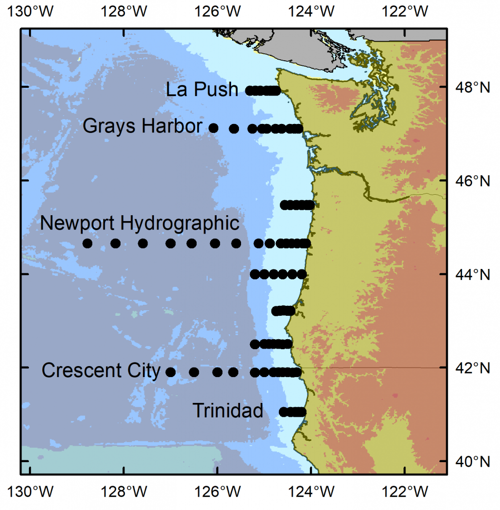
I have just returned from 10 days aboard the NOAA ship Bell M. Shimada, where I was the marine mammal observer on the Northern California Current (NCC) Cruise. These research cruises have sampled the NCC in the winter, spring, and fall for decades. As a result, a wealth of knowledge on the oceanography and plankton community in this dynamic ocean ecosystem has been assimilated by a dedicated team of scientists (find out more via the Newportal Blog). Members of the GEMM Lab have joined this research effort in the past two years, conducting marine mammal surveys during the transits between sampling stations (Fig. 2).
Figure 2. Northern California Current cruise sampling locations, where oceanography and plankton data are collected. Marine mammal surveys were conducted on the transits between stations.
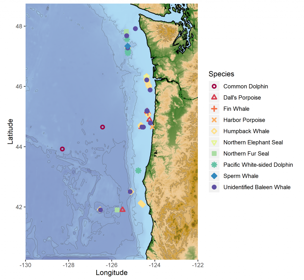
The fall 2019 NCC cruise was a resounding success. We were able to survey a large swath of the ecosystem between Crescent City, CA and La Push, WA, from inshore to 200 miles offshore. During that time, I observed nine different species of marine mammals (Table 1). As often as I use some version of the phrase “the marine environment is patchy and dynamic”, it never fails to sink in a little bit more every time I go to sea. On the map in Fig. 3, note how clustered the marine mammal sightings are. After nearly a full day of observing nothing but blue water, I would find myself scrambling to keep up with recording all the whales and dolphins we were suddenly in the midst of. What drives these clusters of sightings? What is it about the oceanography and prey community that makes any particular area a hotspot for marine mammals? We hope to get at these questions by utilizing the oceanographic data collected throughout the surveys to better understand environmental drivers of these distribution patterns.
Table 1. Summary of marine mammal
sightings from the September 2019 NCC Cruise.
Species
# sightings
Total # individuals
Northern Elephant Seal
1
1
Northern Fur Seal
2
2
Common Dolphin
2
8
Pacific White-sided Dolphin
8
143
Dall’s Porpoise
4
19
Harbor Porpoise
1
3
Sperm Whale
1
1
Fin Whale
1
1
Humpback Whale
22
36
Unidentified Baleen Whale
14
16
Figure 3. Map of marine mammal sighting locations from the September NCC cruise.
It was an auspicious time to survey the Northern California Current. Perhaps you have read recent news reports warning about the formation of another impending marine heatwave, much like the “warm blob” that plagued the North Pacific in 2015. We experienced it first-hand during the NCC cruise, with very warm surface waters off Newport extending out to 200 miles offshore (Fig. 4). A lot of energy input from strong winds would be required to mix that thick, warm layer and allow cool, nutrient-rich water to upwell along the coast. But it is already late September, and as the season shifts from summer to fall we are at the end of our typical upwelling season, and the north winds that would typically drive that mixing are less likely. Time will tell what is in store for the NCC ecosystem as we face the onset of another marine heatwave.
Figure 4. Temperature contours over the upper 150 m from 1-200 miles off Newport, Oregon from Fall 2014-2019. During Fall 2014, the Warm Blob inundated the Oregon shelf. Surface temperatures during that survey were 17°- 18°C along the entire transect. During 2015 and 2016 the warm water (16°C) layer had deepened and occupied the upper 50 m. During 2018, the temperature was 16°C in the upper 20 m and cooler on the shelf, indicative of residual upwelling. During this survey in 2019, we again saw very warm (18°C) temperatures in the upper water column over the entire transect. Image and caption credit: Jennifer Fisher.
It was a joy to spend 10 days at sea with this team of scientists. Insight, collaboration, and innovation are born from interdisciplinary efforts like the NCC cruises. Beyond science, what a privilege it is to be on the ocean with a group of people you can work with and laugh with, from the dock to 200 miles offshore, south to north and back again.
Dawn Barlow on the flying bridge of NOAA Ship Bell M. Shimada, heading out to sea with the Newport bridge in the background. Photo: Anna Bolm.
By Leila Lemos, PhD Candidate, Fisheries and Wildlife Department, Oregon State University
After three years of fieldwork and analyzing a large dataset, it is time to finally start compiling the results, create plots and see what the trends are. The first dataset I am analyzing is the photogrammetry data (more on our photogrammetry method here), which so far has been full of unexpected results.
Our first big expectation was to find a noticeable intra-year variation. Gray whales spend their winter in the warm waters of Baja California, Mexico, period while they are fasting. In the spring, they perform a big migration to higher latitudes. Only when they reach their summer feeding grounds, that extends from Northern California to the Bering and Chukchi seas, Alaska, do they start feeding and gaining enough calories to support their migration back to Mexico and subsequent fasting period.
Northeastern gray whale migration route along the NE Pacific Ocean. Source: https://journeynorth.org/tm/gwhale/annual/map.html
Thus, we expected to see whales arriving along the Oregon coast with a skinny body condition that would gradually improve over the months, during the feeding season. Some exceptions are reasonable, such as a lactating mother or a debilitated individual. However, datasets can be more complex than we expect most of the times, and many variables can influence the results. Our photogrammetry dataset is no different!
In addition, I need to decide what are the best plots to display the results and how to make them. For years now I’ve been hearing about the wonders of R, but I’ve been skeptical about learning a whole new programming/coding language “just to make plots”, as I first thought. I have always used statistical programs such as SPSS or Prism to do my plots and they were so easy to work with. However, there is a lot more we can do in R than “just plots”. Also, it is not just because something seems hard that you won’t even try. We need to expose ourselves sometimes. So, I decided to give it a try (and I am proud of myself I did), and here are some of the results:
Plot 1: Body Area Index (BAI) vs Day of the Year (DOY)
In this plot, we wanted to assess the annual Body Area Index (BAI) trends that describe how skinny (low number) or fat (higher number) a whale is. BAI is a simplified version of the BMI (Body Mass Index) used for humans. If you are interested about this method we have developed at our lab in collaboration with the Aerial Information Systems Laboratory/OSU, you can read more about it in our publication.
The plots above are three versions of the same data displayed in different ways. The first plot on the left shows all the data points by year, with polynomial best fit lines, and the confidence intervals (in gray). There are many overlapping observation points, so for the middle plot I tried to “clean up the plot” by reducing the size of the points and taking out the gray confidence interval range around the lines. In the last plot on the right, I used a linear regression best fit line, instead of polynomial.
We can see a general trend that the BAI was considerably higher in 2016 (red line), when compared to the following years, which makes us question the accuracy of the dataset for that year. In 2016, we also didn’t sample in the month of July, which is causing the 2016 polynomial line to show a sharp decrease in this month (DOY: ~200-230). But it is also interesting to note that the increasing slope of the linear regression line in all three years is very similar, indicating that the whales gained weight at about the same rate in all years.
Plot 2: Body Area Index (BAI) vs Body Condition Score (BCS)
In addition to the photogrammetry method of assessing whale body condition, we have also performed a body condition scoring method for all the photos we have taken in the field (based on the method described by Bradford et al. 2012). Thus, with this second set of plots, we wanted to compare both methods of assessing whale body condition in order to evaluate when the methods agree or not, and which method would be best and in which situation. Our hypothesis was that whales with a ‘fair’ body condition would have a lower BAI than whales with a ‘good’ body condition.
The plots above illustrate two versions of the same data, with data in the left plot grouped by year, and the data in the right plot grouped by month. In general, we see that no whales were observed with a poor body condition in the last analysis months (August to October), with both methods agreeing to this fact. Additionally, there were many whales that still had a fair body condition in August and September, but less whales in the month of October, indicating that most whales gained weight over the foraging seasons and were ready to start their Southbound migration and another fasting period. This result is important information regarding monitoring and conservation issues.
However, the 2016 dataset is still a concern, since the whales appear to have considerable higher body condition (BAI) when compared to other years.
Plot 3:Temporal Body Area Index (BAI) for individual whales
In this last group of plots, we wanted to visualize BAI trends over the season (using day of year – DOY) on the x-axis) for individuals we measured more than once. Here we can see the temporal patterns for the whales “Bit”, “Clouds”, “Pearl”, “Scarback, “Pointy”, and “White Hole”.
We expected to see an overall gradual increase in body condition (BAI) over the seasons, such as what we can observe for Pointy in 2018. However, some whales decreased their condition, such as Bit in 2018. Could this trend be accurate? Furthermore, what about BAI measurements that are different from the trend, such as Scarback in 2017, where the last observation point shows a lower BAI than past observation points? In addition, we still observe a high BAI in 2016 at this individual level, when compared to the other years.
My next step will be to check the whole dataset again and search for inconsistencies. There is something causing these 2016 values to possibly be wrong and I need to find out what it is. The overall quality of the measured photogrammetry images was good and in focus, but other variables could be influencing the quality and accuracy of the measurements.
For instance, when measuring images, I often struggled with glare, water splash, water turbidity, ocean swell, and shadows, as you can see in the photos below. All of these variables caused the borders of the whale body to not be clearly visible/identifiable, which may have caused measurements to be wrong.
Examples of bad conditions for performing photogrammetry: (1) glare and water splash, (2) water turbidity, (3) ocean swell, and (4) a shadow created in one of the sides of the whale body. Source: GEMM Lab. Taken under NMFS permit 16111 issued to John Calambokidis.
Thus, I will need to check all of these variables to identify the causes for bad measurements and “clean the dataset”. Only after this process will I be able to make these plots again to look at the trends (which will be easy since I already have my R code written!). Then I’ll move on to my next hypothesis that the BAI of individual whales varied by demographics including sex, age and reproductive state.
To carry out robust science that produces results we can trust, we can’t simply collect data, perform a basic analysis, create plots and believe everything we see. Data is often messy, especially when developing new methods like we have done here with drone based photogrammetry and the BAI. So, I need to spend some important time checking my data for accuracy and examining confounding variables that might affect the dataset. Science can be challenging, both when interpreting data or learning a new command language, but it is all worth it in the end when we produce results we know we can trust.
By Alexa Kownacki, Ph.D. Student, OSU Department of Fisheries and Wildlife, Geospatial Ecology of Marine Megafauna Lab
From September 22nd through 30th, the GEMM Lab participated in a STEM research cruise aboard the R/V Oceanus, Oregon State University’s (OSU) largest research vessel, which served as a fully-functioning, floating, research laboratory and field station. The STEM cruise focused on integrating science, technology, engineering and mathematics (STEM) into hands-on teaching experiences alongside professionals in the marine sciences. The official science crew consisted of high school teachers and students, community college students, and Oregon State University graduate students and professors. As with a usual research cruise, there was ample set-up, data collection, data entry, experimentation, successes, and failures. And because everyone in the science party actively participated in the research process, everyone also experienced these successes, failures, and moments of inspiration.
The science party enjoying the sunset from the aft deck with the Astoria-Megler bridge in the background. (Image source: Alexa Kownacki)
Dr. Leigh Torres, Dr. Rachael Orben, and I were all primarily stationed on flybridge—one deck above the bridge—fully exposed to the elements, at the highest possible location on the ship for best viewing. We scanned the seas in hopes of spotting a blow, a splash, or any sign of a marine mammal or seabird. Beside us, students and teachers donned binoculars and positioned themselves around the mast, with Leigh and I taking a 90-degree swath from the mast—either to starboard or to port. For those who had not been part of marine mammal observations previously, it was a crash course into the peaks and troughs—of both the waves and of the sightings. We emphasized the importance of absence data: knowledge of what is not “there” is equally as important as what is. Fortunately, Leigh chose a course that proved to have surprisingly excellent environmental conditions and amazing sightings. Therefore, we collected a large amount of presence data: data collected when marine mammals or seabirds are present.
High school student, Chris Quashnick Holloway, records a seabird sighting for observer, Dr. Rachael Orben. (Image source: Alexa Kownacki).
When someone sighted a whale that surfaced regularly, we assessed the conditions: the sea state, the animal’s behavior, the wind conditions, etc. If we deemed them as “good to fly”, our licensed drone pilot and Orange Coast Community College student, Jason, prepared his Phantom 4 drone. While he and Leigh set up drone operations, I and the other science team members maintained a visual on the whale and stayed in constant communication with the bridge via radio. When the drone was ready, and the bridge gave the “all clear”, Jason launched his drone from the aft deck. Then, someone tossed an unassuming, meter-long, wood plank overboard—keeping it attached to the ship with a line. This wood board serves as a calibration tool; the drone flies over it at varying heights as determined by its built-in altimeter. Later, we analyze how many pixels one meter occupied at different heights and can thereby determine the body length of the whale from still images by converting pixel length to a metric unit.
High school student, Alishia Keller, uses binoculars to observe a whale, while PhD student, Alexa Kownacki, radios updates on the whale’s location to the bridge and the aft deck. (Image source: Tracy Crews)
Finally, when the drone is calibrated, I radio the most recent location of our animal. For example, “Blow at 9 o’clock, 250 meters away”. Then, the bridge and I constantly adjust the ship’s speed and location. If the whale “flukes” (dives and exposes the ventral side of its tail), and later resurfaced 500 meters away at our 10 o’clock, I might radio to the bridge to, “turn 60 degrees to port and increase speed to 5 knots”. (See the Hidden Math Lesson below). Jason then positions the drone over the whale, adjusting the camera angle as necessary, and recording high-quality video footage for later analysis. The aerial viewpoint provides major advantages. Whales usually expose about 10 percent of their body above the water’s surface. However, with an aerial vantage point, we can see more of the whale and its surroundings. From here, we can observe behaviors that are otherwise obscured (Torres et al. 2018), and record footage that to help quantify body condition (i.e. lengths and girths). Prior to the batteries running low, Jason returns the drone back to the aft deck, the vessel comes to an idle, and Leigh catches the drone. Throughout these operations, those of us on the flybridge photograph flukes for identification and document any behaviors we observe. Later, we match the whale we sighted to the whale that the drone flew over, and then to prior sightings of this same individual—adding information like body condition or the presence of a calf. I like to think of it as whale detective work. Moreover, it is a team effort; everyone has a critical role in the mission. When it’s all said and done, this noninvasive approach provides life history context to the health and behaviors of the animal.
Drone pilot, Jason Miranda, flying his drone using his handheld ground station on the aft deck. (Photo source: Tracy Crews)
Hidden Math Lesson: The location of 10 o’clock and 60 degrees to port refer to the exact same direction. The bow of the ship is our 12 o’clock with the stern at our 6 o’clock; you always orient yourself in this manner when giving directions. The same goes for a compass measurement in degrees when relating the direction to the boat: the bow is 360/0. An angle measure between two consecutive numbers on a clock is: 360 degrees divided by 12-“hour” markers = 30 degrees. Therefore, 10 o’clock was 0 degrees – (2 “hours”)= 0 degrees- (2*30 degrees)= -60 degrees. A negative degree less than 180 refers to the port side (left).
Killer whale traveling northbound.
Our trip was chalked full of science and graced with cooperative weather conditions. There were more highlights than I could list in a single sitting. We towed zooplankton nets under the night sky while eating ice cream bars; we sang together at sunset and watched the atmospheric phenomena: the green flash; we witnessed a humpback lunge-feeding beside the ship’s bow; and we saw a sperm whale traveling across calm seas.
Sperm whale surfacing before a long dive.
On this cruise, our lab focused on the marine mammal observations—which proved excellent during the cruise. In only four days of surveying, we had 43 marine mammal sightings containing 362 individuals representing 9 species (See figure 1). As you can see from figure 2, we traveled over shallow, coastal and deep waters, in both Washington and Oregon before inland to Portland, OR. Because we ventured to areas with different bathymetric and oceanographic conditions, we increased our likelihood of seeing a higher diversity of species than we would if we stayed in a single depth or area.
Humpback whale lunge feeding off the bow.
Number of sightings
Total number of individuals
Humpback whale
22
40
Pacific white-sided dolphin
3
249
Northern right whale dolphin
1
9
Killer whale
1
3
Dall’s porpoise
5
49
Sperm whale
1
1
Gray whale
1
1
Harbor seal
1
1
California sea lion
8
9
Total
43
362
Figure 1. Summary table of all species sightings during cruise while the science team observed from the flybridge.
Pacific white-sided dolphins swimming towards the vessel.
Figure 2. Map with inset displaying study area and sightings observed by species during the cruise, made in ArcMap. (Image source: Alexa Kownacki).
Even after two days of STEM outreach events in Portland, we were excited to incorporate more science. For the transit from Portland, OR to Newport, OR, the entire science team consisted two people: me and Jason. But even with poor weather conditions, we still used science to answer questions and help us along our journey—only with different goals than on our main leg. With the help of the marine technician, we set up a camera on the bow of the ship, facing aft to watch the vessel maneuver through the famous Portland bridges.
Video 1. Time-lapse footage of the R/V Oceanus maneuvering the Portland Bridges from a GoPro. Compiled by Alexa Kownacki, assisted by Jason Miranda and Kristin Beem.
Prior to the crossing the Columbia River bar and re-entering the Pacific Ocean, the R/V Oceanus maneuvered up the picturesque Columbia River. We used our geospatial skills to locate our fellow science team member and high school student, Chris, who was located on land. We tracked each other using GPS technology in our cell phones, until the ship got close enough to use natural landmarks as reference points, and finally we could use our binoculars to see Chris shining a light from shore. As the ship powered forward and passed under the famous Astoria-Megler bridge that connects Oregon to Washington, Chris drove over it; he directed us “100 degrees to port”. And, thanks to clear directions, bright visual aids, and spatiotemporal analysis, we managed to find our team member waving from shore. This is only one of many examples that show how in a few days at sea, students utilized new skills, such as marine mammal observational techniques, and honed them for additional applications.
On the bow, Alexa and Jason use binoculars to find Chris–over 4 miles–on the Washington side of the Columbia River. (Image source: Kristin Beem)
Great science is the result of teamwork, passion, and ingenuity. Working alongside students, teachers, and other, more-experienced scientists, provided everyone with opportunities to learn from each other. We created great science because we asked questions, we passed on our knowledge to the next person, and we did so with enthusiasm.
High school students, Jason and Chris, alongside Dr. Leigh Torres, all try to get a glimpse at the zooplankton under Dr. Kim Bernard’s microscope. (Image source: Tracy Crews).
Check out other blog posts written by the science team about the trip here.
By Alexa Kownacki, Ph.D. Student, OSU Department of Fisheries and Wildlife, Geospatial Ecology of Marine Megafauna Lab
Did you know that Excel has a maximum number of rows? I do. During Winter Term for my GIS project, I was using Excel to merge oceanographic data, from a publicly-available data source website, and Excel continuously quit. Naturally, I assumed I had caused some sort of computer error. [As an aside, I’ve concluded that most problems related to technology are human error-based.] Therefore, I tried reformatting the data, restarting my computer, the program, etc. Nothing. Then, thanks to the magic of Google, I discovered that Excel allows no more than 1,048,576 rows by 16,384 columns. ONLY 1.05 million rows?! The oceanography data was more than 3 million rows—and that’s with me eliminating data points. This is what happens when we’re dealing with big data.
According to Merriam-Webster dictionary, big data is an accumulation of data that is too large and complex for processing by traditional database management tools (www.merriam-webster.com). However, there are journal articles, like this one from Forbes, that discuss the ongoing debate of how to define “big data”. According to the article, there are 12 major definitions; so, I’ll let you decide what you qualify as “big data”. Either way, I think that when Excel reaches its maximum row capacity, I’m working with big data.
Collecting oceanography data aboard the R/V Shimada. Photo source: Alexa K.
Here’s the thing: the oceanography data that I referred to was just a snippet of my data. Technically, it’s not even MY data; it’s data I accessed from NOAA’s ERDDAP website that had been consistently observed for the time frame of my dolphin data points. You may recall my blog about maps and geospatial analysis that highlights some of the reasons these variables, such as temperature and salinity, are important. However, what I didn’t previously mention was that I spent weeks working on editing this NOAA data. My project on common bottlenose dolphins overlays environmental variables to better understand dolphin population health off of California. These variables should have similar spatiotemporal attributes as the dolphin data I’m working with, which has a time series beginning in the 1980s. Without taking out a calculator, I still know that equates to a lot of data. Great data: data that will let me answer interesting, pertinent questions. But, big data nonetheless.
This is a screenshot of what the oceanography data looked like when I downloaded it to Excel. This format repeats for nearly 3 million rows.
Excel Screen Shot. Image source: Alexa K.
I showed this Excel spreadsheet to my GIS professor, and his response was something akin to “holy smokes”, with a few more expletives and a look of horror. It was not the sheer number of rows that shocked him; it was the data format. Nowadays, nearly everyone works with big data. It’s par for the course. However, the way data are formatted is the major split between what I’ll call “easy” data and “hard” data. The oceanography data could have been “easy” data. It could have had many variables listed in columns. Instead, this data alternated between rows with variable headings and columns with variable headings, for millions of cells. And, as described earlier, this is only one example of big data and its challenges.
Data does not always come in a form with text and numbers; sometimes it appears as media such as photographs, videos, and audio files. Big data just got a whole lot bigger. While working as a scientist at NOAA’s Southwest Fisheries Science Center, one project brought in over 80 terabytes of raw data per year. The project centered on the eastern north pacific gray whale population, and, more specifically, its migration. Scientists have observed the gray whale migration annually since 1994 from Piedras Blancas Light Station for the Northbound migration, and 2 out of every 5 years from Granite Canyon Field Station (GCFS) for the Southbound migration. One of my roles was to ground-truth software that would help transition from humans as observers to computer as observers. One avenue we assessed was to compare how well a computer “counted” whales compared to people. For this question, three infrared cameras at the GCFS recorded during the same time span that human observers were counting the migratory whales. Next, scientists, such as myself, would transfer those video files, upwards of 80 TB, from the hard drives to Synology boxes and to a different facility–miles away. Synology boxes store arrays of hard drives and that can be accessed remotely. To review, three locations with 80 TB of the same raw data. Once the data is saved in triplet, then I could run a computer program, to detect whale. In summary, three months of recorded infrared video files requires upwards of 240 TB before processing. This is big data.
Scientists on an observation shift at Granite Canyon Field Station in Northern California. Photo source: Alexa K.
Alexa and another NOAA scientist watching for gray whales at Piedras Blancas Light Station. Photo source: Alexa K.
In the GEMM Laboratory, we have so many sources of data that I did not bother trying to count. I’m entering my second year of the Ph.D. program and I already have a hard drive of data that I’ve backed up three different locations. It’s no longer a matter of “if” you work with big data, it’s “how”. How will you format the data? How will you store the data? How will you maintain back-ups of the data? How will you share this data with collaborators/funders/the public?
The wonderful aspect to big data is in the name: big and data. The scientific community can answer more, in-depth, challenging questions because of access to data and more of it. Data is often the limiting factor in what researchers can do because increased sample size allows more questions to be asked and greater confidence in results. That, and funding of course. It’s the reason why when you see GEMM Lab members in the field, we’re not only using drones to capture aerial images of whales, we’re taking fecal, biopsy, and phytoplankton samples. We’re recording the location, temperature, water conditions, wind conditions, cloud cover, date/time, water depth, and so much more. Because all of this data will help us and help other scientists answer critical questions. Thus, to my fellow scientists, I feel your pain and I applaud you, because I too know that the challenges that come with big data are worth it. And, to the non-scientists out there, hopefully this gives you some insight as to why we scientists ask for external hard drives as gifts.
Leila launching the drone to collect aerial images of gray whales to measure body condition. Photo source: Alexa K.
Using the theodolite to collect tracking data on the Pacific Coast Feeding Group in Port Orford, OR. Photo source: Alexa K.
By Alexa Kownacki, Ph.D. Student, OSU Department of Fisheries and Wildlife, Geospatial Ecology of Marine Megafauna Lab
The first lecture slide. Source: Lecture1_Population Dynamics_Lou Botsford
This was the very first lecture slide in my population dynamics course at UC Davis. Population dynamics was infamous in our department for being an ultimate rite of passage due to its notoriously challenging curriculum. So, when Professor Lou Botsford pointed to his slide, all 120 of us Wildlife, Fish, and Conservation Biology majors, didn’t know how to react. Finally, he announced, “This [pointing to the slide] is all of you”. The class laughed. Lou smirked. Lou knew.
Lou knew that there is more truth to this meme than words could express. I can’t tell you how many times friends and acquaintances have asked me if I was going to be a park ranger. Incredibly, not all—or even most—wildlife biologists are park rangers. I’m sure that at one point, my parents had hoped I’d be holding a tiger cub as part of a conservation project—that has never happened. Society may think that all wildlife biologists want to walk in the footsteps of the famous Steven Irwin and say thinks like “Crikey!”—but I can’t remember the last time I uttered that exclamation with the exception of doing a Steve Irwin impression. Hollywood may think we hug trees—and, don’t get me wrong, I love a good tie-dyed shirt—but most of us believe in the principles of conservation and wise-use A.K.A. we know that some trees must be cut down to support our needs. Helicoptering into a remote location to dart and take samples from wild bear populations…HA. Good one. I tell myself this is what I do sometimes, and then the chopper crashes and I wake up from my dream. But, actually, a scientist staring at a computer with stacks of papers spread across every surface, is me and almost every wildlife biologist that I know.
The “dry lab” on the R/V Nathaniel B. Palmer en route to Antarctica. This room full of technology is where the majority of the science takes place. Drake Passage, International Waters in August 2015. Source: Alexa Kownacki
There is an illusion that wildlife biologists are constantly in the field doing all the cool, science-y, outdoors-y things while being followed by a National Geographic photojournalist. Well, let me break it to you, we’re not. Yes, we do have some incredible opportunities. For example, I happen to know that one lab member (eh-hem, Todd), has gotten up close and personal with wild polar bear cubs in the Arctic, and that all of us have taken part in some work that is worthy of a cover image on NatGeo. We love that stuff. For many of us, it’s those few, memorable moments when we are out in the field, wearing pants that we haven’t washed in days, and we finally see our study species AND gather the necessary data, that the stars align. Those are the shining lights in a dark sea of papers, grant-writing, teaching, data management, data analysis, and coding. I’m not saying that we don’t find our desk work enjoyable; we jump for joy when our R script finally runs and we do a little dance when our paper is accepted and we definitely shed a tear of relief when funding comes through (or maybe that’s just me).
A picturesque moment of being a wildlife biologist: Alexa and her coworker, Jim, surveying migrating gray whales. Piedras Blancas Light Station, San Simeon, CA in May 2017. Source: Alexa Kownacki.
What I’m trying to get at is that we accepted our fates as the “scientists in front of computers surrounded by papers” long ago and we embrace it. It’s been almost five years since I was a senior in undergrad and saw this meme for the first time. Five years ago, I wanted to be that scientist surrounded by papers, because I knew that’s where the difference is made. Most people have heard the quote by Mahatma Gandhi, “Be the change that you wish to see in the world.” In my mind, it is that scientist combing through relevant, peer-reviewed scientific papers while writing a compelling and well-researched article, that has the potential to make positive changes. For me, that scientist at the desk is being the change that he/she wish to see in the world.
Scientists aboard the R/V Nathaniel B. Palmer using the time in between net tows to draft papers and analyze data…note the facial expressions. Antarctic Peninsula in August 2015. Source: Alexa Kownacki.
One of my favorite people to colloquially reference in the wildlife biology field is Milton Love, a research biologist at the University of California Santa Barbara, because he tells it how it is. In his oh-so-true-it-hurts website, he has a page titled, “So You Want To Be A Marine Biologist?” that highlights what he refers to as, “Three really, really bad reasons to want to be a marine biologist” and “Two really, really good reasons to want to be a marine biologist”. I HIGHLY suggest you read them verbatim on his site, whether you think you want to be a marine biologist or not because they’re downright hilarious. However, I will paraphrase if you just can’t be bothered to open up a new tab and go down a laugh-filled wormhole.
Really, Really Bad Reasons to Want to be a Marine Biologist:
To talk to dolphins. Hint: They don’t want to talk to you…and you probably like your face.
You like Jacques Cousteau. Hint: I like cheese…doesn’t mean I want to be cheese.
Hint: Lack thereof.
Really, Really Good Reasons to Want to be a Marine Biologist:
Work attire/attitude. Hint: Dress for the job you want finally translates to board shorts and tank tops.
You like it. *BINGO*
Alexa with colleagues showing the “cool” part of the job is working the zooplankton net tows. This DOES have required attire: steel-toed boots, hard hat, and float coat. R/V Nathaniel B. Palmer, Antarctic Peninsula in August 2015. Source: Alexa Kownacki.
In summary, as wildlife or marine biologists we’ve taken a vow of poverty, and in doing so, we’ve committed ourselves to fulfilling lives with incredible experiences and being the change we wish to see in the world. To those of you who want to pursue a career in wildlife or marine biology—even after reading this—then do it. And to those who don’t, hopefully you have a better understanding of why wearing jeans is our version of “business formal”.
A fieldwork version of a lab meeting with Leigh Torres, Tom Calvanese (Field Station Manager), Florence Sullivan, and Leila Lemos. Port Orford, OR in August 2017. Source: Alexa Kownacki.
This summer was full of emotions for me: I finally started my first fieldwork season after almost a year of classes and saw my first gray whale (love at first sight!).
During the fieldwork we use a small research vessel (we call it “Red Rocket”) along the Oregon coast to collect data for my PhD project. We are collecting gray whale fecal samples to analyze hormone variations; acoustic data to assess ambient noise changes at different locations and also variations before, during and after events like the “Halibut opener”; GoPro recordings to evaluate prey availability; photographs in order to identify each individual whale and assess body and skin condition; and video recordings through UAS (aka “drone”) flights, so we can measure the whales and classify them as skinny/fat, calf/juvenile/adult and pregnant/non-pregnant.
However, in order to collect all of these data, we need to first find the whales. This is when we use our first sense: vision. We are always looking at the horizon searching for a blow to come up and once we see it, we safely approach the animal and start watching the individual’s behavior and taking photographs.
If the animal is surfacing regularly to allow a successful drone overflight, we stay with the whale and launch the UAS in order to collect photogrammetry and behavior data.
Each team member performs different functions on the boat, as seen in the figure below.
Figure 1: UAS image showing each team members’ functions in the boat at the moment just after the UAS launch.
While one member pilots the boat, another operates the UAS. Another team member is responsible for taking photos of the whales so we can match individuals with the UAS videos. And the last team member puts the calibration board of known length in the water, so that we can later calculate the exact size of each pixel at various UAS altitudes, which allows us to accurately measure whale lengths. Team members also alternate between these and other functions.
Sometimes we put the UAS in the air and no whales are at the surface, or we can’t find any. These animals only stay at the surface for a short period of time, so working with whales can be really challenging. UAS batteries only last for 15-20 minutes and we need to make the most of that time as we can. All of the members need to help the UAS pilot in finding whales, and that is when, besides vision, we need to use hearing too. The sound of the whale’s respiration (blow) can be very loud, especially when whales are closer. Once we find the whale, we give the location to the UAS pilot: “whale at 2 o’clock at 30 meters from the boat!” and the pilot finds the whale for an overflight.
The opposite – too many whales around – can also happen. While we are observing one individual or searching for it in one direction, we may hear a blow from another whale right behind us, and that’s the signal for us to look for other individuals too.
But now you might be asking yourself: “ok, I agree with vision and hearing, but what about the other three senses? Smell? Taste? Touch?” Believe it or not, this happens. Sometimes whales surface pretty close to the boat and blow. If the wind is in our direction – ARGHHHH – we smell it and even taste it (after the first time you learn to close your mouth!). Not a smell I recommend.
Fecal samples are responsible for the 5th sense: touch!
Once we identify that the whale pooped, we approach the fecal plume in order to collect as much fecal matter as possible (Fig.2).
Figure 2: A: the poop is identified; B: the boat approaches the feces that are floating at the surface (~30 seconds); C: one of the team members remains at the bow of the boat to indicate where the feces are; D: another team member collects it with a fine-mesh net. Filmed under NOAA/NMFS permit #16111 to John Calambokidis).
After collecting the poop we transfer all of it from the net to a small jar that we then keep cool in an ice chest until we arrive back at the lab and put it in the freezer. So, how do we transfer the poop to the jar? By touching it! We put the jar inside the net and transfer each poop spot to the jar with the help of water pressure from a squeeze bottle full of ambient salt water.
Figure 3: Two gray whale individuals swimming around kelp forests. Filmed under NOAA/NMFS permit #16111 to John Calambokidis).
That’s how we use our senses to study the whales, and we also use an underwater sensory system (a GoPro) to see what the whales were feeding on.
GoPro video of mysid swarms that we recorded near feeding gray whales in Port Orford in August 2016:
Our fieldwork is wrapping up this week, and I can already say that it has been a success. The challenging Oregon weather allowed us to work on 25 days: 6 days in Port Orford and 19 days in the Newport and Depoe Bay region, totaling 141 hours and 50 minutes of effort. We saw 195 whales during 97 different sightings and collected 49 fecal samples. We also performed 67 UAS flights, 34 drifter deployments (to collect acoustic data), and 34 GoPro deployments.
It is incredible to see how much data we obtained! Now starts the second part of the challenge: how to put all of this data together and find the results. My next steps are:
– photo-identification analysis;
– body and skin condition scoring of individuals;
– photogrammetry analysis;
– analysis of the GoPro videos to characterize prey;
– hormone analysis laboratory training in November at the Seattle Aquarium
For now, enjoy some pictures and a video we collected during the fieldwork this summer. It was hard to choose my favorite pictures from 11,061 photos and a video from 13 hours and 29 minutes of recording, but I finally did! Enjoy!
Figure 4: Gray whale breaching in Port Orford on August 27th. (Photo by Leila Lemos; Taken under NOAA/NMFS permit #16111 to John Calambokidis).
Figure 5: Rainbow formation through sunlight refraction on the water droplets of a gray whale individual’s blow in Newport on September 15th. (Photo by Leila Lemos; Taken under NOAA/NMFS permit #16111 to John Calambokidis).
Likely gray whale nursing behavior (Taken under NOAA/NMFS permit #16111 to John Calambokidis):
**GUEST POST**written by Cheyenne Coleman of Savannah State University
My first journey to the west coast, was spent on a six hour flight to Portland, Oregon in anticipation of my upcoming summer internship with the Geospatial Ecology and Marine Megafuana lab (GEMM Lab) at the Hatfield Marine Science Center (HMSC). I had never before been to the west coast, but luckily for me I did not have to make this long journey alone; my friend, Kamiliya Daniels, was also doing an internship at HMSC. After a long bus ride to Corvallis, Kamiliya and I, were warmly greeted by one of my GEMM lab members, Amanda Holdman. With her, was honorary GEMM lab member and Amanda’s dog, Boiler, who spent the greater part of the drive to Newport sleeping on my lap while I spent the drive asking Amanda several series of questions,
“Are there bears in these woods?”
“What do the dorms look like? How do I get around town? I hear it’s a small town, is there at least a Walmart?”
But without any answer to my curiosity, all of these questions were left with one reply:
“I’ll let you see for yourself.”
And then just as Amanda proposed, I did exactly that.
My name is Cheyenne and I am from Savannah State University in Georgia interning with LMRCSC (Living Marine Resources Cooperative Science Center) in Newport, Oregon. My expectations of the Oregon coast and the reality was vastly different than what I had pictured. I imagined the entire West Coast would match a California summer; Sunny and hot.
But on the contrary, upon arrival to Newport, I learned, it doesn’t. It is windy and chilly and hardly ever above 70 degrees. Thinking an Oregon summer would match a California summer, in my suitcase I possessed only three small sweaters and an abundant supply of shorts and tank tops. Needless, to say I was quickly off to buy an Oregon Coast sweatshirt that would double as warmth and a souvenir. Upon first entering Newport, I was mostly shocked at how small the town felt, and I noticed every structure was made of wood, and coming from Georgia this was strange to me. In Georgia, everything is made of bricks and cement. The dorms on first glance reminded me of summer camp for adults: slightly dated with bunk bed sleeping arrangements. Yikes!
However, my worries that come along with moving to a new place, were quickly diminished when I was welcomed to the GEMM lab; Florence greeted with a warm cup of tea, I was introduced to everyone who worked at HMSC, and even given my very own desk in the GEMM lab. After a day of transitions, and a much needed good night’s rest, I was introduced to my project on California Sea Lions (Zalophus californianus).
If you’ve been following along with all of the latest posts from GEMM lab students, you might think the lives of spatial ecologists revolve around glamorous fieldwork. We’ve got Amanda eavesdropping on porpoises, Florence surveying for foraging gray whales, and Leigh playing hide and seek with seabirds down in Yachats. I, however, am admittedly not spending my summer in the field this year and am learning that there is more to being a scientist than picturesque moments with charismatic study species in beautiful locations.
Prior to entering the GEMM lab, I had limited experience in computing and data analysis and spent my prior summer’s doing fieldwork on invertebrates, usually bagging sediment and collecting water samples. This internship was a new and unique opportunity for me to learn the next step of the scientific process. While I had always wondered, “What happens after data collection?” I was not given the experience to find out. I quickly learned, that this includes a lot of sorting, categorizing, and modeling, all of which are very time consuming.
By using satellite tracking information of California sea lions collected by the Oregon Department of Fish and Wildlife (ODFW) from 2005 and 2007, I am able to measure movements and habitat use of California sea lions. By analyzing their routes between their initial and final locations, we can study their distributions patterns.
To some people, sitting at a computer doing analysis may not seem as glamorous as working in the field. Some people might question why someone would chose to spend their career in front of a computer screen. But my internship this summer, really showed me the value of having experience working at all stages of the scientific process. Seeing all of my efforts in processing, sorting, and categorizing come together to create an end result really enhanced my love for science. By connecting the questions to the answers, and making contributions to the scientific community, I feel rewarded for my hard work.
My internship has come to an end, and given my initial hesitations, I’ve grown accustomed to Newport and the GEMM lab. I enjoy sitting at my desk running through a wild assortment of data and hearing the wonderful ding of the teapot. In the last days of my internship, I was able to escape my computer screen to assist Florence in data collection on beautiful gray whale surveys. Last Thursday, a lab meeting was held and my lab mates and I were able to update each other on our research. We shared ideas on how to enhance everyone’s project, and who might be able to answer questions we were struggling with in our own data sets. As my internship comes to a close, I have gained more knowledge and real life skill then I would ever hope to gain just through courses at Savannah State. I learned new software programs like R Statistical Package and sharpened my own skills in ArcGIS. I gained the experience of collaborating with a lab, and understanding how powerful working with your peers and colleagues can be. Gaining this much experience has, without a doubt, given me an edge in the competitive field I will enter after graduation. I have made connections, hopefully life long, with the nicest people; I know that in the future, which ever path I may choose, I’ll always be a part of the GEMM lab.


You must be logged in to post a comment.