By Leila S. Lemos, PhD Candidate in Wildlife Sciences, Fisheries and Wildlife Department, OSU
As you might know, the GEMM Lab (Geospatial Ecology of MARINE Megafauna Laboratory) researches the marine environment, but today I am going to leave the marine ecosystem aside and I will discuss the Amazon biome. As a Brazilian, I cannot think of anything else to talk about this week than the terrifying fire that is burning down the Amazon forest in this exact minute.
For some context, the Amazon biome is known as the biome with the highest biodiversity in the world (ICMBio, 2019). It is the largest biome in Brazil, accounting for ~49% of the Brazilian territory. This biome houses the biggest tropical forest and hydrographic basin in the world. The Amazon forest also extends through eight other countries: Bolivia, Colombia, Ecuador, Guiana, French Guiana, Peru, Suriname and Venezuela. To date, at least 40,000 plant species, 427 mammals, 1,300 birds, 378 reptiles, more than 400 amphibians, around 3,000 freshwater fishes, and around 100,000 invertebrate species have been described by scientists in the Amazon, comprising more than 1/3 of all fauna species on the planet (Da Silva et al. 2005, Lewinsohn and Prado 2005). And, these numbers are likely to increase; According to Patterson (2000), one new genus and eight new species of Neotropical mammals are discovered each year in the region.
I feel very connected to the Amazon as I worked as an environmental consultant and field coordinator in 2014 and 2015 (Figs. 1 and 2) along the Madeira river (or “Wood” river) in Rondonia, Brazil (Fig. 3). I monitored Amazon river dolphins (Inia geoffrensis; Fig. 4), a species considered endangered by the IUCN Red List in 2018 (Da Silva et al. 2018). The Madeira river originates in Bolivia and flows into the great Amazon river, comprising one of its main tributaries (Fig. 3).
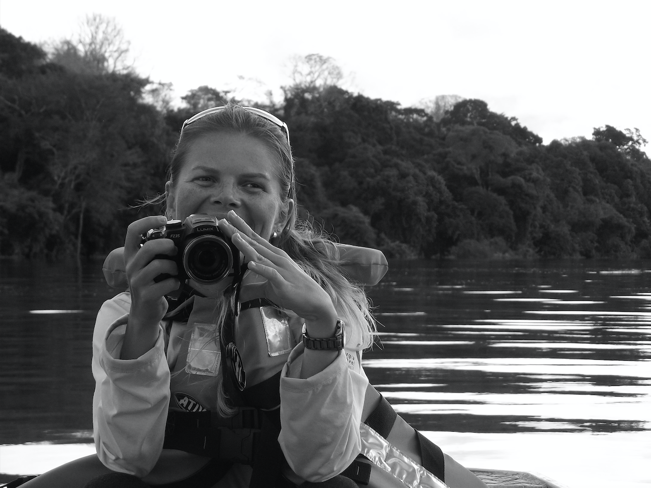
Source: Laura K. Honda, 2015.
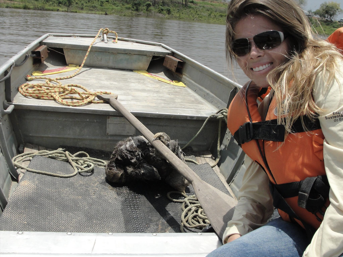
Source: Roberta Lanziani, 2014.
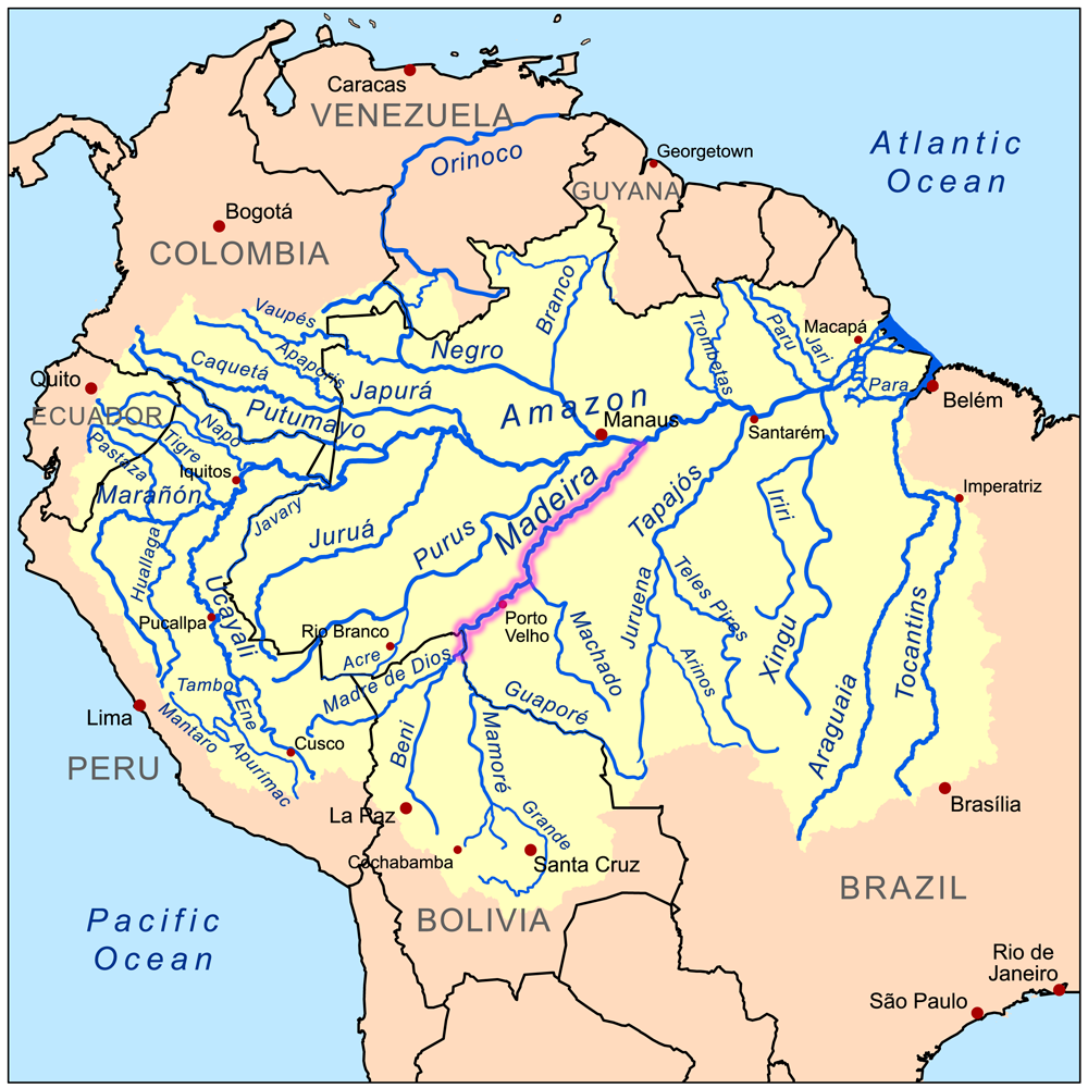
Source: Wikipedia, 2019.
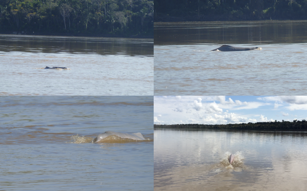
Source: Leila S. Lemos, 2014; 2015.
Here is also a video where you can see some Amazon river dolphins along the Madeira river:
Source: Leila S. Lemos, 2014; 2015.
In addition to the dolphins, I witnessed the presence of many other fauna specimens like birds (including macaws and parrots), monkeys, alligators and sloths (Fig. 5). The biodiversity of the Amazon is unquestionable.
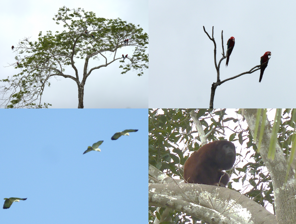
Source: Leila S. Lemos
Other than its great biodiversity, the Amazon is known as the “lungs of the Earth”, which is an erroneous statement since plants consume as much oxygen as they produce (Malhi et al. 2008, Malhi 2019). But still, the Amazon forest is responsible for 16% of the oxygen produced by photosynthesis on land and 9% of the oxygen on the global scale (Fig. 6). This seems a small percentage, but it is still substantial, especially because the plants use carbon dioxide during photosynthesis, which accounts for a 10% reduction of atmospheric carbon dioxide. Thus, imagine if there was no Amazon rainforest. The rise in carbon dioxide would be enormous and have serious implications on the global climate, surpassing safe temperature boundaries for many regions.
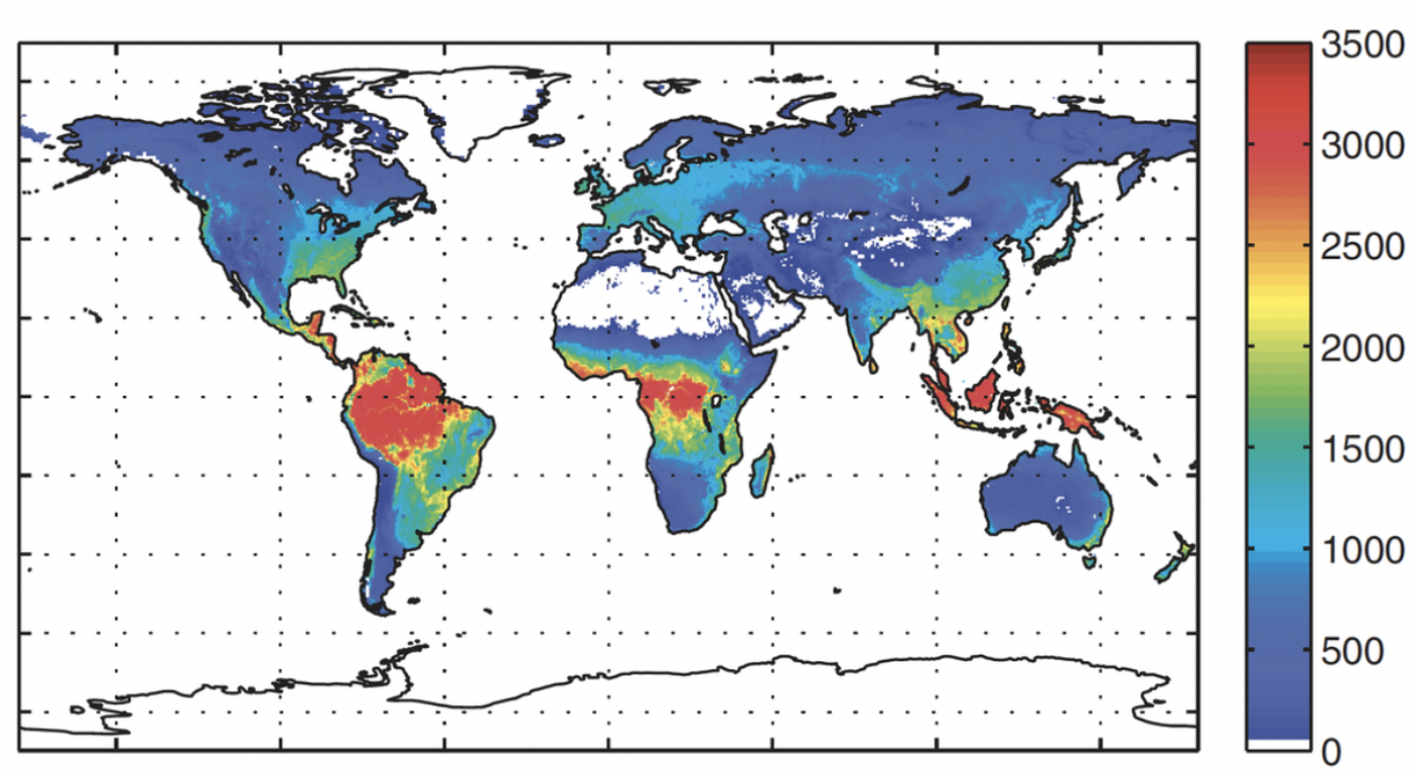
Source: Malhi 2019.
Unfortunately, this scenario is not really far from us. Even though deforestation indices have fallen in the last 15 years, fire incidence associated with droughts and carbon emissions have increased (Aragão et al. 2018; Fig. 7).
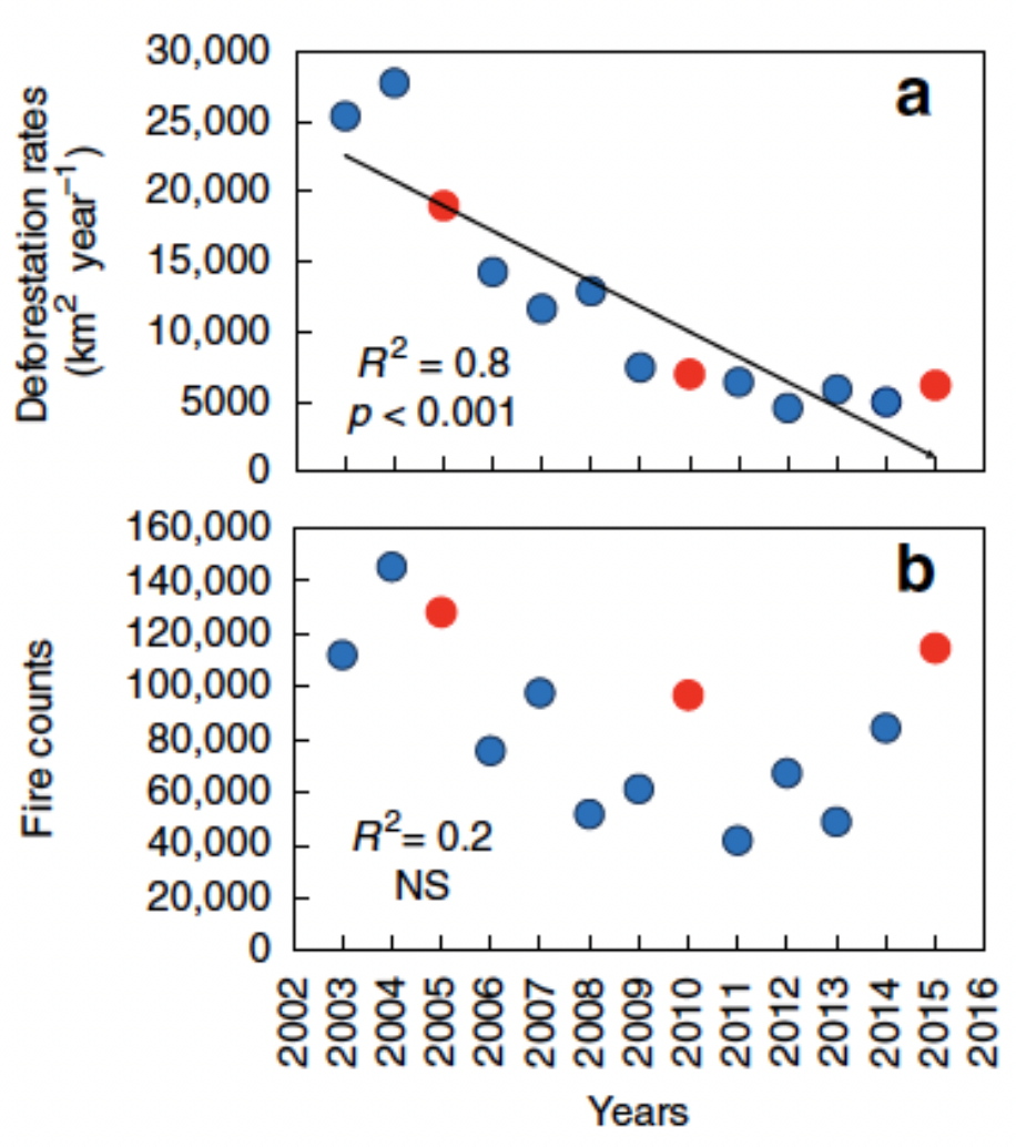
Source: Aragão et al. 2018.
Since August 2019, the Amazon forest has experienced extreme fire outbreaks (Figs. 8 and 9). Around 80,000 fires occurred only in 2019. Despite 2019 not being an extreme drought year, the period of January-August 2019 is characterized by an ~80% increase in fires compared to the previous year (Wagner and Hayes 2019). The intensification of the fires has been linked to the Brazilian President’s incentive to “open the rainforest to development”. Leaving politics aside, the truth is that the majority of these fires have been set by loggers and ranchers seeking to clear land to expand the agro-cattle area (Yeung 2019).
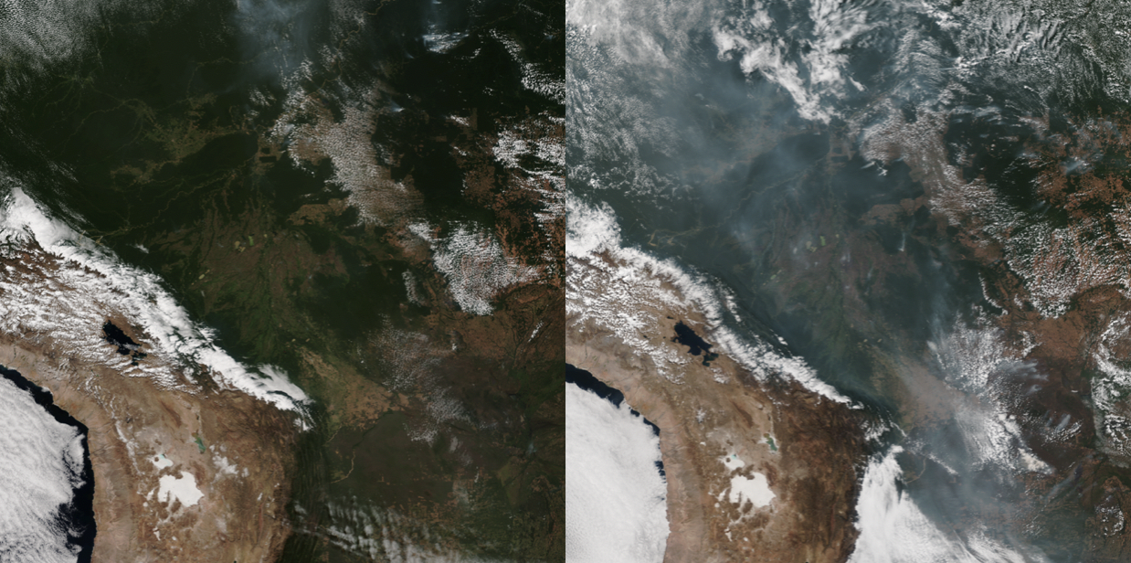
Source: NOAA, in: Wagner and Hayes, 2019.
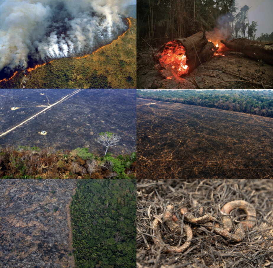
Source: Buzz Feed News 2019, Sea Mashable 2019.
Here you can see some videos showing the extension of the problem:
Video 1 – by NBC News:
Video 2 – a drone footage by The Guardian:
I consider myself lucky for the opportunity to have worked in the Amazon rainforest before these chaotic fires have destroyed so much biodiversity. The Amazon is a crucial home for countless animal and plant species, and to ~900,000 indigenous individuals that live in the region. They are all at risk of losing their homes and lives. We are all at risk of global warming.
References
Aragão LEOC, Anderson LO, Fonseca MG, Rosan TM, Vedovato LB, Wagner FH, Silva CVJ, Silva Junior CHL, Arai E, Aguiar AP, Barlow J, Berenguer E, Deeter MN, Domingues LG, Gatti L, Gloor M, Malhi Y, Marengo JA, Miller JB, Phillips OL, and Saatchi S. 2018. 21stCentury drought-related fires counteract the decline of Amazon deforestation carbon emissions. Nature Communications 9(536):1-12.
Buzz Feed News. 2019. These Heartbreaking Photos Show The Devastation Of The Amazon Fires. Retrieved 1 September 2019 from https://www.buzzfeednews.com/article/gabrielsanchez/photos-trending-devastation-amazon-wildfire
Da Silva JMC, Rylands AB, and Da Fonseca GAB. 2005. The Fate of the Amazonian Areas of Endemism. Conservation Biology 19(3):689-694.
Da Silva V, Trujillo F, Martin A, Zerbini AN, Crespo E, Aliaga-Rossel E, and Reeves R. 2018. Inia geoffrensis. The IUCN Red List of Threatened Species 2018: e.T10831A50358152. http://dx.doi.org/10.2305/IUCN.UK.2018-2.RLTS.T10831A50358152.en. Downloaded on 27 August 2019.
ICMBio. 2019. Amazônia. Retrieved 26 August 2019 from http://www.icmbio.gov.br/portal/unidades deconservacao/biomas-brasileiros/amazonia
Lewinsohn TM, and Prado PI. 2005. How Many Species Are There in Brazil? Conservation Biology 19(3):619.
Malhi Y. 2019. does the amazon provide 20% of our oxygen? Travels in ecosystem science. Retrieved 29 August 2019 from http://www.yadvindermalhi.org/blog/does-the-amazon-provide-20-of-our-oxygen
Malhi Y., Roberts JT, Betts RA, Killeen TJ, Li W, Nobre CA. 2008. Climate Change, Deforestation, and the Fate of the Amazon. Science 319:169-172.
Patterson BD. 2000. Patterns and trends in the discovery of new Neotropical mammals. Diversity and Distributions, 6, 145-151.
Sea Mashable. 2019. The Amazon forest is burning to the ground. Here’s how it happened and what you can do to help. Retrieved 1 September 2019 from https://sea.mashable.com/culture/5813/the-amazon-forest-is-burning-to-the-ground-heres-how-it-happened-and-what-you-can-do-to-help
Wagner M, and Hayes M. 2019. Wildfires rage in the Amazon. CNN. Retrieved 26 August 2019 from https://www.cnn.com/americas/live-news/amazon-wildfire-august-2019/index.html
Wikipedia. 2019. Madeira river. Retrieved 29 August 2019 from https://en.wikipedia.org/wiki/Madeira_River
Yeung J. 2019. Blame humans for starting the Amazon fires, environmentalists say. CNN. Retrieved 26 August 2019 from https://www.cnn.com/2019/08/22/americas/amazon-fires-humans-intl-hnk-trnd/index.html


You must be logged in to post a comment.