Can sea otters help kelp under a changing climate?

By Dominique Kone1 and Sara Hamilton2

1Masters Student in Marine Resource Management, 2Doctoral Student in Integrative Biology

Five years ago, the North Pacific Ocean experienced a sudden increase in sea surface temperature (SST), known as the warm blob, which altered marine ecosystem function and structure (Leising et al. 2015). Much research illustrated how the warm blob impacted pelagic ecosystems, with relatively less focused on the nearshore environment. Yet, a new study demonstrated how rising ocean temperatures have partially led to bull kelp loss in northern California. Unfortunately, we are once again observing similar warming trends, representing the second largest marine heatwave over recent decades, and signaling the potential rise of a second warm blob. Taken together, all these findings could forecast future warming-related ecosystem shifts in Oregon, highlighting the need for scientists and managers to consider strategies to prevent future kelp loss, such as reintroducing sea otters.

In northern California, researchers observed a dramatic ecosystem shift from productive bull kelp forests to purple sea urchin barrens. The study, led by Dr. Laura Rogers-Bennett from the University of California, Davis and California Department of Fish and Wildlife, determined that this shift was caused by multiple climatic and biological stressors. Beginning in 2013, sea star populations were decimated by sea star wasting disease (SSWD). Sea stars are a main predator of urchins, causing their absence to release purple urchins from predation pressure. Then, starting in 2014, ocean temperatures spiked with the warm blob. These two events created nutrient-poor conditions, which limited kelp growth and productivity, and allowed purple urchin populations to grow unchecked by predators and increase grazing on bull kelp. The combined effect led to approximately 90% reductions in bull kelp, with a reciprocal 60-fold increase in purple urchins (Figure 1).

Figure 1. Kelp loss and ecosystem shifts in northern California (Rogers-Bennett & Catton 2019).

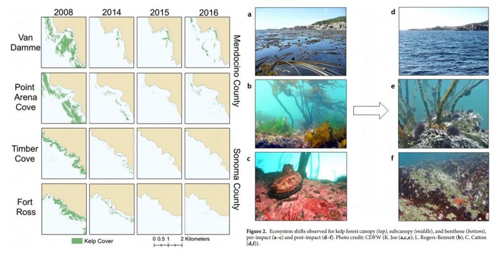
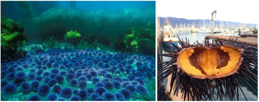
These changes have wrought economic challenges as well as ecological collapse in Northern California. Bull kelp is important habitat and food source for several species of economic importance including red abalone and red sea urchins (Tegner & Levin 1982). Without bull kelp, red abalone and red sea urchin populations have starved, resulting in the subsequent loss of the recreational red abalone ($44 million) and commercial red sea urchin fisheries in Northern California. With such large kelp reductions, purple urchins are also now in a starved state, evidenced by noticeably smaller gonads (Rogers-Bennett & Catton 2019).

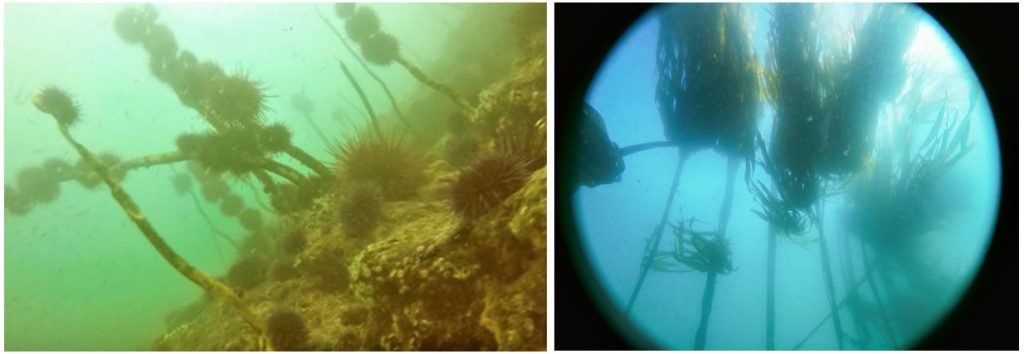
Biogeographically, southern Oregon is very similar to northern California, as both are composed of complex rocky substrates and shorelines, bull kelp canopies, and benthic macroinvertebrates (i.e. sea urchins, abalone, etc.). Because Oregon was also impacted by the 2014-2015 warm blob and SSWD, we might expect to see a similar coastwide kelp forest loss along our southern coastline. The story is more complicated than that, however. For instance, ODFW has found purple urchin barrens where almost no kelp remains in some localized places. The GEMM Lab has video footage of purple urchins climbing up kelp stalks to graze within one of these barrens near Port Orford, OR (Figure 2, left). In her study, Dr. Rogers-Bennett explains that this aggressive sea urchin feeding strategy is potentially a sign of food limitation, where high-density urchin populations create intense resource competition. Conversely, at sites like Lighthouse Reef (~45 km from Port Orford) outside Charleston, OR, OSU and University of Oregon divers are currently seeing flourishing bull kelp forests. Urchins at this reef have fat, rich gonads, which is an indicator of high-quality nutrition (Figure 2, right).

Satellites can detect kelp on the surface of the water, giving scientists a way to track kelp extent over time. Preliminary results from Sara Hamilton’s Ph.D. thesis research finds that while some kelp forests have shrunk in past years, others are currently bigger than ever in the last 35 years. It is not clear what is driving this spatial variability in urchin and kelp populations, nor why southern Oregon has not yet faced the same kind of coastwide kelp forest collapse as northern California. Regardless, it is likely that kelp loss in both northern California and southern Oregon may be triggered and/or exacerbated by rising temperatures.

Figure 2. Left: Purple urchin aggressive grazing near Port Orford, OR (GEMM Lab 2019). Right: Flourishing bull kelp near Charleston, OR (Sara Hamilton 2019).

The reintroduction of sea otters has been proposed as a solution to combat rising urchin populations and bull kelp loss in Oregon. From an ecological perspective, there is some validity to this idea. Sea otters are a voracious urchin predator that routinely reduce urchin populations and alleviate herbivory on kelp (Estes & Palmisano 1974). Such restoration and protection of bull kelp could help prevent red abalone and red sea urchin starvation. Additionally, restoring apex predators and increasing species richness is often linked to increased ecosystem resilience, which is particularly important in the face of global anthropogenic change (Estes et al. 2011)

While sea otters could alleviate grazing pressure on Oregon’s bull kelp, this idea only looks at the issue from a top-down, not bottom-up, perspective. Sea otters require a lot of food (Costa 1978, Reidman & Estes 1990), and what they eat will always be a function of prey availability and quality (Ostfeld 1982). Just because urchins are available, doesn’t mean otters will eat them. In fact, sea otters prefer large and heavy (i.e. high gonad content) urchins (Ostfeld 1982). In the field, researchers have observed sea otters avoiding urchins at the center of urchin barrens (personal communication), presumably because those urchins have less access to kelp beds than on the barren periphery, and therefore, are constantly in a starved state (Konar & Estes 2003) (Figure 3). These findings suggest prey quality is more important to sea otter survival than just prey abundance.

Figure 3. Left: Sea urchin barren (Annie Crawley). Right: Urchin gonads (Sea to Table).

Purple urchin quality has not been widely assessed in Oregon, but early results show that gonad size varies widely depending on urchin density and habitat type. In places where urchin barrens have formed, like Port Orford, purple urchins are likely starving and thus may be a poor source of nutrition for sea otters. Before we decide whether sea otters are a viable tool to combat kelp loss, prey surveys may need to be conducted to assess if a sea otter population could be sustained based on their caloric requirements. Furthermore, predictions of how these prey populations may change due to rising temperatures could help determine the potential for sea otters to become reestablished in Oregon under rapid environmental change.

Recent events in California could signal climate-driven processes that are already impacting some parts of Oregon and could become more widespread. Dr. Rogers-Bennett’s study is valuable as she has quantified and described ecosystem changes that might occur along Oregon’s southern coastline. The resurgence of a potential second warm blob and the frequency between these warming events begs the question if such temperature spikes are still anomalous or becoming the norm. If the latter, we could see more pronounced kelp loss and major shifts in nearshore ecosystem baselines, where function and structure is permanently altered. Whether reintroducing sea otters can prevent these changes will ultimately depend on prey and habitat availability and quality, and should be carefully considered.

References:

Costa, D. P. 1978. The ecological energetics, water, and electrolyte balance of the California sea otter (Enhydra lutris). Ph.D. dissertation, University of California, Santa Cruz.

Estes, J. A. and J.F. Palmisano. 1974. Sea otters: their role in structuring nearshore communities. Science. 185(4156): 1058-1060.

Estes et al. 2011. Trophic downgrading of planet Earth. Science. 333(6040): 301-306.

Harvell et al. 2019. Disease epidemic and a marine heat wave are associated with the continental-scale collapse of a pivotal predator (Pycnopodia helianthoides). Science Advances. 5(1).

Konar, B., and J. A. Estes. 2003. The stability of boundary regions between kelp beds and deforested areas. Ecology. 84(1): 174-185.

Leising et al. 2015. State of California Current 2014-2015: impacts of the warm-water “blob”. CalCOFI Reports. (56): 31-68.

Ostfeld, R. S. 1982. Foraging strategies and prey switching in the California sea otter. Oecologia. 53(2): 170-178.

Reidman, M. L. and J. A. Estes. 1990. The sea otter (Enhydra lutris): behavior, ecology, and natural history. United States Department of the Interior, Fish and Wildlife Service, Biological Report. 90: 1-126.

Rogers-Bennett, L., and C. A. Catton. 2019. Marine heat wave and multiple stressors tip bull kelp forest to sea urchin barrens. Scientific Reports. 9:15050.

Tegner, M. J., and L. A. Levin. 1982. Do sea urchins and abalones compete in California? International Echinoderms Conference, Tampa Bay. J. M Lawrence, ed.

Whispers of fear

By Leila S. Lemos, Ph.D. candidate in Wildlife Sciences, Fisheries and Wildlife Department


What did you do when playing hide-and-seek? You would try your best not to move or make any noise that would cause the seeker to hear you and find you, right? So, I always associated the prey-predator relationship to a hide-and-seek game, where prey hide, and predators seek. Thus, if you are the prey in this food chain game you should try to hide and not make any noise.

I read an article last week that made me think of this relationship again. The article, “Right whale moms ‘whisper’ to their babies so sharks won’t hear”, announced the study findings from Susan E. Parks and collaborators (2019), which really called my attention.

To give some context, North Atlantic Right Whales (NARWs; Eubalaena glacialis; Fig. 1) occur primarily in northern Atlantic coastal waters or close to the continental shelf (Fig. 2), yet their presence in deep waters are also known (NOAA 2019).

Figure 1: A mother-calf pair of North Atlantic right whales.
Source: Dana Cusano, Syracuse University (NMFS Permit #775-1875); retrieved from Kooser 2019.

Figure 2: North Atlantic right whale distribution.
Source: NOAA 2019.

The species is critically endangered and estimated at less than 500 individuals (IUCN 2007, Pace et al. 2017). Unlike several other whale populations, NARWs have not rebounded from intense whaling, and its population has begun to decrease since 2010 (Thomas et al. 2016, Pace et al. 2017). NARWs’ biggest threats are associated with anthropogenic activities, including entanglement in fishing lines and collisions with vessels (Fig. 3).

Figure 3: North Atlantic right whales’ biggest threats: (A) entanglement in fishing gear, and (B) vessel collision.
Source (A): Peter Duley (NOAA), retrieved from Guy 2017; (B) Williams 2019.

Other than anthropogenic impacts, NARWs also face natural threats like predation. There are reports on newborn and young right whale calf’s predation by killer whales and large sharks (Taylor et al. 2013, Parks et al. 2019; Fig. 4).

Figure 4: Mother carries her calf carcass presenting two semicircular shark bite marks on its flank.
Source: Taylor et al. 2013.

Whales communicate by acoustic signals that can efficiently propagate underwater and be detected by listening predators (Parks et al. 2019). It is possible that mother-calf pairs may use cryptic behaviors to avoid the attention of predators by shifting their communication patterns, leading to a hypothesis that they produce low-amplitude calls and lower call rates (Tyack 2000; Fig. 5). These two behavioral modifications have been previously observed in mother-calf pairs of humpback whales (Megaptera novaeangliae; Videsen et al. 2017) and southern right whales (Eubalaena australis; Nielsen et al. 2019).

Figure 5: Spectrogram and waveform of a single pulse (low amplitude) and an upcall (high amplitude) produced by a right whale. A louder and longer signal (high-amplitude call) is potentially easier to detect by predators.
Source: Parks et al. 2019.

In order to determine if NARWs exhibited the same behavior, Parks and collaborators (2019) tagged lactating and non-lactating females, and a pregnant female that later was tagged again with her calf, to collect acoustic, movement and orientation data. Their results indicate that lactating females use a significantly higher low-amplitude call rate (mean ± standard deviation: 7.13 ± 2.0 calls) when compared to high-amplitude calls (0.88 ± 0.70 calls). In contrast, non-lactating females exhibited higher rates of high-amplitude calls (3.21 ± 2.29 calls) and lower rates of calls of low-amplitude (0.80 ± 1.15 calls).

Even though their sample size was small (n = 16), the authors had more lactating females sampled than the other demographic groups (n = 11), and their results provide evidence that right whale mother-calf pairs exhibit a shift in their repertoire: Mother-calf pairs reduce high-amplitude calls as compared with other demographic groups in the same habitat (Fig. 6).

Figure 6: Proportion of high and low-amplitude calls by both lactating and non-lactating female right whales on the calving grounds located in the southeastern United States.
Source: Parks et al. 2019.

According to Dr. Parks, these low-amplitude sounds are analogous with human whispers (Kooser, 2019). This ‘whispering’ is a behavioral adaptation that allows communication between mother and calf without drawing the attention of undesirable predators.

Such an adaptation may seem obvious to us when we think back of our hide-and-seek game, but documentation of little details of the cryptic lives of whales is unique and fascinating.  We still don’t know so much about the lives of whales, so determining adaptations, behavioral and physiological changes, and other simple features like “whispering” are crucial for us to better understand the ‘whale world’ and be able to enhance conservation efforts.


References

Guy 2017. North Atlantic right whales are going extinct. A new invention could save them. Retrieved from https://oceana.org/blog/north-atlantic-right-whales-are-going-extinct-new-invention-could-save-them. Accessed on 17 Oct 2019.

IUCN 2007. North Atlantic Right Whale. Retrieved from https://www.iucnredlist.org/species/41712/10541234. Accessed on 16 Oct 2019.

Kooser A. 2019. Right whale moms ‘whisper’ to their babies so sharks won’t hear. CNET. Retrieved from https://www.cnet.com/news/right-whale-moms-whisper-to-their-babies-for-an-important-reason/?fbclid=IwAR0JcKgYPII4a-BTjm7VPtOfjyVIb63F-SLAjyZZ2KXA6GvYJozfazcfHjA. Accessed on 16 Oct 2019.

Nielsen ML, Bejder L, Videsen SK, Christiansen F, Madsen PT. 2019. Acoustic crypsis in southern right whale mother-calf pairs: infrequent, low-output calls to avoid predation? J. Exp. Biol. 222:jeb190728.

NOAA 2019. North Atlantic Right Whale. NOAA Fisheries. Retrieved from https://www.fisheries.noaa.gov/species/north-atlantic-right-whale. Accessed on 16 Oct 2019.

Pace III RM, Corkeron PJ, Kraus SD. 2017. State-space mark-recapture estimates reveal a recent decline in abundance of North Atlantic right whales. Ecology and Evolution 7:8730–8741.

Parks SE, Cusano DA, Van Parijs SM, Nowacek DP. 2019. Acoustic crypsis in communication by North Atlantic right whale mother-calf pairs on the calving grounds. Biology Letters 15:20190485.

Taylor JKD, Mandelman JW, McLellan WA, Moore MJ, Skomal GB, Rotstein DS, Kraus SD. 2013. Shark predation on North Atlantic right whales (Eubalaena glacialis) in the southeastern United States calving ground. Marine Mammal Science 29(1): 204–212.

Thomas PO, Reeves RR, Brownell RL. 2016. Status of the world baleen whales. Marine Mammal Science 32:682–734.

Tyack PL. 2000. Functional aspects of cetacean communication. In Cetacean societies: field studies of dolphins and whales (eds J Mann, RC Connor, PL Tyack, H Whitehead), pp. 270–307. Chicago, IL:University of Chicago Press.

Videsen SKA, Bejder L, Johnson M, Madsen PT. 2017. High suckling rates and acoustic crypsis of humpback whale neonates maximise potential for mother-calf energy transfer. Funct. Ecol. 31:1561–1573.

Williams 2019. Right whale grandmother known as Punctuation killed by ship strike. Retrieved from https://www.cbc.ca/news/canada/nova-scotia/north-atlantic-right-whale-punctuation-died-after-ship-strike-1.5191987. Accessed on 17 Oct 2019.

Demystifying the algorithm

By Clara Bird, Masters Student, OSU Department of Fisheries and Wildlife, Geospatial Ecology of Marine Megafauna Lab

Hi everyone! My name is Clara Bird and I am the newest graduate student in the GEMM lab. For my master’s thesis I will be using drone footage of gray whales to study their foraging ecology. I promise to talk about how cool gray whales in a following blog post, but for my first effort I am choosing to write about something that I have wanted to explain for a while: algorithms. As part of previous research projects, I developed a few semi-automated image analysis algorithms and I have always struggled with that jargon-filled phrase. I remember being intimidated by the term algorithm and thinking that I would never be able to develop one. So, for my first blog I thought that I would break down what goes into image analysis algorithms and demystify a term that is often thrown around but not well explained.

What is an algorithm?

The dictionary broadly defines an algorithm as “a step-by-step procedure for solving a problem or accomplishing some end” (Merriam-Webster). Imagine an algorithm as a flow chart (Fig. 1), where each step is some process that is applied to the input(s) to get the desired output. In image analysis the output is usually isolated sections of the image that represent a specific feature; for example, isolating and counting the number of penguins in an image. Algorithm development involves figuring out which processes to use in order to consistently get desired results. I have conducted image analysis previously and these processes typically involve figuring out how to find a certain cutoff value. But, before I go too far down that road, let’s break down an image and the characteristics that are important for image analysis.

Figure 1. An example of a basic algorithm flow chart. There are two inputs: variables A and B. The process is the calculation of the mean of the two variables.

What is an image?

Think of an image as a spread sheet, where each cell is a pixel and each pixel is assigned a value (Fig. 2). Each value is associated with a color and when the sheet is zoomed out and viewed as a whole, the image comes together.  In color imagery, which is also referred to as RGB, each pixel is associated with the values of the three color bands (red, green, and blue) that make up that color. In a thermal image, each pixel’s value is a temperature value. Thinking about an image as a grid of values is helpful to understand the challenge of translating the larger patterns we see into something the computer can interpret. In image analysis this process can involve using the values of the pixels themselves or the relationships between the values of neighboring pixels.

Figure 2. A diagram illustrating how pixels make up an image. Each pixel is a grid cell associated with certain values. Image Source: https://web.stanford.edu/class/cs101/image-1-introduction.html

Our brains take in the whole picture at once and we are good at identifying the objects and patterns in an image. Take Figure 3 for example: an astute human eye and brain can isolate and identify all the different markings and scars on the fluke. Yet, this process would be very time consuming. The trick to building an algorithm to conduct this work is figuring out what processes or tools are needed to get a computer to recognize what is marking and what is not. This iterative process is the algorithm development.

Figure 3. Photo ID image of a gray whale fluke.

Development

An image analysis algorithm will typically involve some sort of thresholding. Thresholds are used to classify an image into groups of pixels that represent different characteristics. A threshold could be applied to the image in Figure 3 to separate the white color of the markings on the fluke from the darker colors in the rest of the image. However, this is an oversimplification, because while it would be pretty simple to examine the pixel values of this image and pick a threshold by hand, this threshold would not be applicable to other images. If a whale in another image is a lighter color or the image is brighter, the pixel values would be different enough from those in the previous image for the threshold to inaccurately classify the image. This problem is why a lot of image analysis algorithm development involves creating parameterized processes that can calculate the appropriate threshold for each image.

One successful method used to determine thresholds in images is to first calculate the frequency of color in each image, and then apply the appropriate threshold. Fletcher et al. (2009) developed a semiautomated algorithm to detect scars in seagrass beds from aerial imagery by applying an equation to a histogram of the values in each image to calculate the threshold. A histogram is a plot of the frequency of values binned into groups (Fig. 4). Essentially, it shows how many times each value appears in an image. This information can be used to define breaks between groups of values. If the image of the fluke were transformed to a gray scale, then the values of the marking pixels would be grouped around the value for white and the other pixels would group closer to black, similar to what is shown in Figure 4. An equation can be written that takes this frequency information and calculates where the break is between the groups. Since this method calculates an individualized threshold for each image, it’s a more reliable method for image analysis. Other characteristics could also be used to further filter the image, such as shape or area.

However, that approach is not the only way to make an algorithm applicable to different images; semi-automation can also be helpful. Semi-automation involves some kind of user input. After uploading the image for analysis, the user could also provide the threshold, or the user could crop the image so that only the important components were maintained. Keeping with the fluke example, the user could crop the image so that it was only of the fluke. This would help reduce the variety of colors in the image and make it easier to distinguish between dark whale and light marking.

Figure 4. Example histogram of pixel values. Source: Moallem et al. 2012

Why algorithms are important

Algorithms are helpful because they make our lives easier. While it would be possible for an analyst to identify and digitize each individual marking from a picture of a gray whale, it would be extremely time consuming and tedious. Image analysis algorithms significantly reduce the time it takes to process imagery. A semi-automated algorithm that I developed to count penguins from still drone imagery can count all the penguins on a one km2 island in about 30 minutes, while it took me 24 long hours to count them by hand (Bird et al. in prep). Furthermore, the process can be repeated with different imagery and analysts as part of a time series without bias because the algorithm eliminates human error introduced by different analysts.

Whether it’s a simple combination of a few processes or a complex series of equations, creating an algorithm requires breaking down a task to its most basic components. Development involves translating those components step by step into an automated process, which after many trials and errors, achieves the desired result. My first algorithm project took two years of revising, improving, and countless trials and errors.  So, whether creating an algorithm or working to understand one, don’t let the jargon nor the endless trials and errors stop you. Like most things in life, the key is to have patience and take it one step at a time.

References

Bird, C. N., Johnston, D.W., Dale, J. (in prep). Automated counting of Adelie penguins (Pygoscelis adeliae) on Avian and Torgersen Island off the Western Antarctic Peninsula using Thermal and Multispectral Imagery. Manuscript in preparation

Fletcher, R. S., Pulich, W. ‡, & Hardegree, B. (2009). A Semiautomated Approach for Monitoring Landscape Changes in Texas Seagrass Beds from Aerial Photography. https://doi.org/10.2112/07-0882.1

Moallem, Payman & Razmjooy, Navid. (2012). Optimal Threshold Computing in Automatic Image Thresholding using Adaptive Particle Swarm Optimization. Journal of Applied Research and Technology. 703.

What does it mean to be an effective science communicator?

By Dominique Kone, Masters Student in Marine Resource Management

To succeed as a scientist, you not only need to be well-trained in the scientific method, but also be familiar with the standards and practices in your discipline. While many scientists are skilled in the production of scientific information, fewer are as well-prepared to disseminate and communicate that information to diverse audiences. As a graduate student, learning effective science communication is one of my top priorities because I believe scientific information can and should be accessible to everyone. As I’ve been building and expanding upon my own communication toolbox, I constantly ask myself, what is effective science communication?

Simply put, communication can be thought of as the two-way transfer of information and knowledge. On one side, information is broadcasted and amplified out into the world, and on the other side, that information is received and understood, ideally. If communicating were this easy, people would never have to worry about being misinterpreted. Yet, this ideal is far from reality, and information is oftentimes misconstrued and/or ignored. This scenario is quite common when scientists communicate technical concepts or findings to non-scientists, either due to differences in communication styles or terminology use. In connecting with these types of audiences, I think effective science communication is a function of three key qualities: intentionality, creativity, and knowledge.

Source: ISTOCKPHOTO/THINKSTOCK

Intentionality

When scientists communicate information, being intentional with what they say and when they say it, can greatly influence how messages resonate with their audience. There’s often a big disconnect between the very specific scientific terms scientists use and the terms their non-technical audiences use. One way scientists can bridge this disconnect and be more intentional (thoughtful), is with word-choice. When scientists change their words, this doesn’t mean they “dumb down” their presentations; rather, they substitute words to better explain concepts in terms the audience easily understands. For example, if I tell the public “I’m predicting sea otter populations at carrying capacity in Oregon using a Bayesian habitat model”, this sentence has three jargon words (carrying capacity, Bayesian, model) that likely mean nothing to this audience. Instead, what I say is, “I’m predicting how many sea otters could live in Oregon based on available habitat”. Now I’m speaking in terms that resonate with my audience, and I have effectively made the same point. An intentional science communicator knows how to deliver information to meet their audience’s ability to take in and process that information.

Source: Andrew Grossman

Creativity

Scientists typically follow structured and defensible protocols when conducting analyses. Far fewer standards apply to how they communicate that research, which can free them up to be more creative in their delivery. One way scientists can be both intentional and creative is by using analogies, examples, or metaphors. When I give talks, I always talk about the high metabolism of sea otters (30% of their own body weight in food, daily) (Costa 1978, Riedman & Estes 1990). Most researchers seem intrigued by this fact, but anyone younger than the age of 10, honestly, could care less. To catch their attention, I always follow up this fact by estimating how many pizza slices I would need to eat to reach that daily food requirement, based on my own weight (230 pizza slices, if you’re curious). By using this analogy, my young audience not only understands my point, but they’re now way more interested because they can’t fathom a human eating that much pizza. It’s a simple comparison, but effective.

Creativity can also be applied to the different ways scientific information is delivered. Scientists regularly publish their work in peer-review scientific journals to reach other scientists. But they also produce short reports and fact sheets to briefly summarize studies for managers or policy-makers. They hold events or workshops to engage stakeholders. They use blogs, webpages, and YouTube to reach the broader public. They even use Twitter to share papers! Scientists do so much more than just publishing their work, and they have several options for delivering and communicating their research. All these different options create more opportunities for scientists to experiment and find new and exciting ways to deliver their science.

A stoic scientist communicating to the masses. Source: Dave Allen via NIWA.

Knowledge

It’s important for scientists to be knowledgeable about their subjects when communicating, but they can’t know everything. Rather, I think a more reasonable goal is for scientists to be comfortable and prepared to say what they know and what they don’t know. Scientists have a thirst for knowledge, but some communicate false information because they have a drive to answer every question they’re asked. They can sometimes get into trouble when they’re asked to talk about something they’re less familiar with. When asked a difficult question, I’ve witnessed a lot of scientists say, “I don’t know”, or, “I don’t know, but I could speculate [insert answer] based on other information”.  This response allows them to answer the question, while also being truthful. The alternative could have real negative implications (e.g. a certain President spreading false information about a dangerous hurricane).

Aside from factual knowledge, contextual knowledge is underappreciated in science communication, but can be vitally important. Some management issues are politically contentious, and effective science communicators can play vital roles in those management processes or actions. One study found that by scientists engaging with stakeholders in the planning process for renewable energy development along the coast of Maine, community members felt the development planning process was being conducted in the most effective manner (Johnson et al. 2015). In this example, a seemingly contentious situation was defused because scientists understood the political and social landscape, and were able to carefully communicate with stakeholders before any management actions took place. Scientists are not required to engage with stakeholders to this degree, but being sensitive to the broader (political, social, cultural, economic) environment in which those stakeholders live and operate can help them better target your messages and relieve potential tension.

GEMM Lab booth at Hatfield Marine Science Day! Source: Leila Lemos.

These three qualities (intentionality, creativity, and knowledge) are not meant to serve as hard, fast science communication rules. Instead, these are simply some qualities I’ve observed in other scientists skilled in effective communication. Scientists don’t automatically enter this space as expert communicators. For those that are great at it, it probably took some time and practice to hone their skills and find their own voice. It might come more naturally to some scientists, but I would argue most – like myself – have to work really hard to develop those skills. As I progress through my career, I’m excited to develop my own skills in effective science communication, and perhaps discover new and exciting approaches along the way.

References:

Costa, D. P. 1978. The ecological energetics, water, and electrolyte balance of the California sea otter (Enhydra lutris). Ph.D. dissertation, University of California, Santa Cruz.

Reidman, M. L. and J. A. Estes. 1990. The sea otter (Enhydra lutris): behavior, ecology, and natural history. United States Department of the Interior, Fish and Wildlife Service, Biological Report. 90: 1-126.

Johnson, T. R., Jansujwiez, J. S., and G. Zydlewski. 2015. Tidal power development n Maine: stakeholder identification and perceptions of engagement. Estuaries and Coasts 38: S266-S278.

Burning it down

By Leila S. Lemos, PhD Candidate in Wildlife Sciences, Fisheries and Wildlife Department, OSU

As you might know, the GEMM Lab (Geospatial Ecology of MARINE Megafauna Laboratory) researches the marine environment, but today I am going to leave the marine ecosystem aside and I will discuss the Amazon biome. As a Brazilian, I cannot think of anything else to talk about this week than the terrifying fire that is burning down the Amazon forest in this exact minute.

For some context, the Amazon biome is known as the biome with the highest biodiversity in the world (ICMBio, 2019). It is the largest biome in Brazil, accounting for ~49% of the Brazilian territory. This biome houses the biggest tropical forest and hydrographic basin in the world. The Amazon forest also extends through eight other countries: Bolivia, Colombia, Ecuador, Guiana, French Guiana, Peru, Suriname and Venezuela. To date, at least 40,000 plant species, 427 mammals, 1,300 birds, 378 reptiles, more than 400 amphibians, around 3,000 freshwater fishes, and around 100,000 invertebrate species have been described by scientists in the Amazon, comprising more than 1/3 of all fauna species on the planet (Da Silva et al. 2005, Lewinsohn and Prado 2005). And, these numbers are likely to increase; According to Patterson (2000), one new genus and eight new species of Neotropical mammals are discovered each year in the region.

I feel very connected to the Amazon as I worked as an environmental consultant and field coordinator in 2014 and 2015 (Figs. 1 and 2) along the Madeira river (or “Wood” river) in Rondonia, Brazil (Fig. 3). I monitored Amazon river dolphins (Inia geoffrensis; Fig. 4), a species considered endangered by the IUCN Red List in 2018 (Da Silva et al. 2018). The Madeira river originates in Bolivia and flows into the great Amazon river, comprising one of its main tributaries (Fig. 3).

Figure 1: Me, working along the Madeira river, Rondonia, Brazil, in 2015.
Source: Laura K. Honda, 2015.

Figure 2: Me, helping to rescue a sloth from the Madeira river, Rondonia, Brazil, in 2014.
Source: Roberta Lanziani, 2014.

Figure 3: The Amazon hydrographic basin, with the Madeira river highlighted.
Source: Wikipedia, 2019.

Figure 4: Amazon river dolphins (I. geoffrensis) along the Madeira river, Rondonia, Brazil.
Source: Leila S. Lemos, 2014; 2015.

Here is also a video where you can see some Amazon river dolphins along the Madeira river:

Source: Leila S. Lemos, 2014; 2015.

In addition to the dolphins, I witnessed the presence of many other fauna specimens like birds (including macaws and parrots), monkeys, alligators and sloths (Fig. 5). The biodiversity of the Amazon is unquestionable.

Figure 5: Macaws (Ara chloropterus), parrots (Amazona sp.) and the Guariba monkey or brown howler (Allouatta guariba) along the Madeira river, Rondonia, Brazil.
Source: Leila S. Lemos

Other than its great biodiversity, the Amazon is known as the “lungs of the Earth”, which is an erroneous statement since plants consume as much oxygen as they produce (Malhi et al. 2008, Malhi 2019). But still, the Amazon forest is responsible for 16% of the oxygen produced by photosynthesis on land and 9% of the oxygen on the global scale (Fig. 6). This seems a small percentage, but it is still substantial, especially because the plants use carbon dioxide during photosynthesis, which accounts for a 10% reduction of atmospheric carbon dioxide. Thus, imagine if there was no Amazon rainforest. The rise in carbon dioxide would be enormous and have serious implications on the global climate, surpassing safe temperature boundaries for many regions.

Figure 6: Total photosynthesis of each major land biome. This value is multiplied by 2.67 to convert to total oxygen production. Hence total oxygen production by photosynthesis on land is around 330 Pg of oxygen per year. The Amazon (just under half of the tropical forests) is around 16% of this, around 54 Pg of oxygen per year.
Source: Malhi 2019.

Unfortunately, this scenario is not really far from us. Even though deforestation indices have fallen in the last 15 years, fire incidence associated with droughts and carbon emissions have increased (Aragão et al. 2018; Fig. 7).

Figure 7: Linear trends (2003–2015) of annual (a) deforestation rates, and (b) active fires counts in the Brazilian Amazon. Red circles indicate the analyzed drought years by Aragão et al. (2018).
Source: Aragão et al. 2018.

Since August 2019, the Amazon forest has experienced extreme fire outbreaks (Figs. 8 and 9). Around 80,000 fires occurred only in 2019. Despite 2019 not being an extreme drought year, the period of January-August 2019 is characterized by an ~80% increase in fires compared to the previous year (Wagner and Hayes 2019). The intensification of the fires has been linked to the Brazilian President’s incentive to “open the rainforest to development”. Leaving politics aside, the truth is that the majority of these fires have been set by loggers and ranchers seeking to clear land to expand the agro-cattle area (Yeung 2019).

Figure 8: The Amazon in July 28: just clouds; and in August 22: choked with smoke.
Source: NOAA, in: Wagner and Hayes, 2019.

Figure 9: Images showing some of the destruction caused by the fires in the Amazon region in 2019.
Source: Buzz Feed News 2019, Sea Mashable 2019.

Here you can see some videos showing the extension of the problem:

Video 1 – by NBC News:

Video 2 – a drone footage by The Guardian:

I consider myself lucky for the opportunity to have worked in the Amazon rainforest before these chaotic fires have destroyed so much biodiversity. The Amazon is a crucial home for countless animal and plant species, and to ~900,000 indigenous individuals that live in the region. They are all at risk of losing their homes and lives. We are all at risk of global warming.

References

Aragão LEOC, Anderson LO, Fonseca MG, Rosan TM, Vedovato LB, Wagner FH, Silva CVJ, Silva Junior CHL, Arai E, Aguiar AP, Barlow J, Berenguer E, Deeter MN, Domingues LG, Gatti L, Gloor M, Malhi Y, Marengo JA, Miller JB, Phillips OL, and Saatchi S. 2018. 21stCentury drought-related fires counteract the decline of Amazon deforestation carbon emissions. Nature Communications 9(536):1-12.

Buzz Feed News. 2019. These Heartbreaking Photos Show The Devastation Of The Amazon Fires. Retrieved 1 September 2019 from https://www.buzzfeednews.com/article/gabrielsanchez/photos-trending-devastation-amazon-wildfire

Da Silva JMC, Rylands AB, and Da Fonseca GAB. 2005. The Fate of the Amazonian Areas of Endemism. Conservation Biology 19(3):689-694.

Da Silva V, Trujillo F, Martin A, Zerbini AN, Crespo E, Aliaga-Rossel E, and Reeves R. 2018. Inia geoffrensis. The IUCN Red List of Threatened Species 2018: e.T10831A50358152. http://dx.doi.org/10.2305/IUCN.UK.2018-2.RLTS.T10831A50358152.en. Downloaded on 27 August 2019.

ICMBio. 2019. Amazônia. Retrieved 26 August 2019 from http://www.icmbio.gov.br/portal/unidades deconservacao/biomas-brasileiros/amazonia

Lewinsohn TM, and Prado PI. 2005. How Many Species Are There in Brazil? Conservation Biology 19(3):619.

Malhi Y. 2019. does the amazon provide 20% of our oxygen? Travels in ecosystem science. Retrieved 29 August 2019 from http://www.yadvindermalhi.org/blog/does-the-amazon-provide-20-of-our-oxygen

Malhi Y., Roberts JT, Betts RA, Killeen TJ, Li W, Nobre CA. 2008. Climate Change, Deforestation, and the Fate of the Amazon. Science 319:169-172.

Patterson BD. 2000. Patterns and trends in the discovery of new Neotropical mammals. Diversity and Distributions, 6, 145-151.

Sea Mashable. 2019. The Amazon forest is burning to the ground. Here’s how it happened and what you can do to help. Retrieved 1 September 2019 from https://sea.mashable.com/culture/5813/the-amazon-forest-is-burning-to-the-ground-heres-how-it-happened-and-what-you-can-do-to-help

Wagner M, and Hayes M. 2019. Wildfires rage in the Amazon. CNN. Retrieved 26 August 2019 from https://www.cnn.com/americas/live-news/amazon-wildfire-august-2019/index.html

Wikipedia. 2019. Madeira river. Retrieved 29 August 2019 from https://en.wikipedia.org/wiki/Madeira_River

Yeung J. 2019. Blame humans for starting the Amazon fires, environmentalists say. CNN. Retrieved 26 August 2019 from https://www.cnn.com/2019/08/22/americas/amazon-fires-humans-intl-hnk-trnd/index.html

Is there life after graduate school?

By Amanda Holdman, MS, GEMM Lab Alumni 2016

I graduated in March 2017 from the GEMM lab at Oregon State, with a Master’s of Science in Wildlife Management. Graduate school was finally over! No more constant coffee refills, popcorn dinners and overnight library stays; I had submitted my final thesis and I was done! Graduate school was no walk in the park for me, and finishing a master’s or a doctorate degree for anyone is no easy feat! It takes years of hard work, commitment, long hours, and a dedication to learning. I remember feeling both excited and a bit disoriented to be done with this phase of much stress and growth. After submitting my thesis, I took a much-needed month off to unknot the muscles in my back and get myself reacquainted with sunlight. The breath of fresh air was exactly what I needed to recover, but it took no time at all for a new type of challenge to emerge: the arduous task of finding a job.

I did what most job seekers do, I sat behind my computer applying for opportunities, hit as many roles as I could, and hoped for the best. Days turned into weeks and weeks turned into months. I was getting desperate, I resorted to applying for a whole spectrum of roles – consulting, project management, administration, youth team leader – hoping that something would land. Soon enough, almost 3 months had passed and I was still in the same spot as before. I was ready to throw in the towel.

In theory, landing a job after graduation sounds like it should be technically easy because more education should mean you are more qualified for the job, but anyone who has been out of grad school for more than an hour can tell you that landing a job after graduate school can be a long and frustrating process. I did not enter this field and its job prospects blindly – that is, I had a working idea of what type of research career I wanted when I completed my education and how much education I would need to get there. I was aware that navigating the job market in a competitive field could be tricky and time-consuming, especially as a green-job seeker. I knew it would be an added difficulty to land a position near the ocean but also close enough to family (I’m from the Midwest). Or at least, I thought I knew how hard it would be to secure a job. The process turned out to be much harder. Mental preparation alone was not enough and months and months of rejection and feeling stuck within the hamster wheel of the job search cycle was becoming my normal.

So, when I was stuck in the depths of a seemingly fruitless job search, and trying as hard as I possibly could, it was hard for me to do anything but roll my eyes, sigh, and give up. But I had to find a way to work through an apparently endless string of rejection by figuring out some way to accept, address and navigate my emotions. I needed to take charge of my own personal development. I started reflecting on what areas of my work on my master’s thesis that I found most difficult and wanted to improve, and would be  an important component of the job I wanted. Identifying my own “knowledge gaps” led me to seek out courses, workshops, job-shadowing and online courses that could fill those holes.

The first thing at the top of my list was to be more efficient at coding. Every job description that made me excited to apply had some description of a coding program: R, Python, MATLAB.  I was lucky enough to attend courses and workshops during my time at the GEMM lab that provided me much of the code I would need to create my habitat models with minimal tweaking. On top of that I was surrounded by supervisors and a lab full of coding geniuses that had an almost, if not completely, open door policy. When I was stuck and a deadline was quickly approaching, it was great to have an army of people to help me get through my obstacles. However, I knew if I wanted to be successful, I needed to become like them: experts and not a beginner. I purchased a subscription to DataCamp, and started searching out courses that could help keep my skills fresh and learn new things. I was over the moon to discover the course “Where are the Fishes?”. It checked all my boxes: geospatial analysis, R, marine related, acoustics…. perfect. Within this course, there were plenty of DataCamp prerequisites, like working with data in the tidyverse and working with dates and times in R, so I had plenty to keep me busy.

I also started looking for in-person, hands-on courses I could enroll in. Since the majority of my marine experience took place on the west coast but I was searching for jobs on the east coast, I enrolled in the Marine Mammal and Sea Turtle Observer Certification Course for the US Atlantic and Gulf of Mexico Oceans in order to learn a little more about identifying species I did not commonly see in nearshore, northern Pacific waters. In this course, I learned about regulations surrounding protected species monitoring, proper camera settings for photographing marine life, and gained the certification needed to work as an observer during seismic surveys for Bureau of Ocean Energy Management (BOEM) and Bureau of Safety and Environmental Enforcement (BSEE) in coordination with the National Marine Fisheries Service. Most of these topics were familiar to me, other than identifying new species, but it was nice to have the refresher and the renewed certification. Heads up this course is coming to Newport in October and I highly recommend it! During this observer course in Charleston, I was able to network with others in the field taking the course, the Charleston aquarium, and the South Carolina DNR. By introducing myself and providing a little bit of my background, I was invited by the South Carolina DNR to watch a satellite tag and release of a sea turtle that the aquarium had been rehabilitating. From the sea turtle release I learned of the International Sea Turtle Symposium that would take place in February in Myrtle Beach, North Carolina and was invited to attend and network by one of the conference chairs, which lead me to my current position. See below…

I tried everything I could to keep myself attached to the field. I attended the Biannual Marine Mammal Conference, enrolled in a bioacoustics short course, watched webinars every Friday, read recent journal articles, looked for voluntary work. I even dropped in on offices like NOAA or Universities of towns I was driving through or visiting to see what they were researching, and if they were looking for researchers. Continuous learning and developing took a lot of time, money, and energy but being conscientious about my personal development kept me motivated and engaged. Graduate school prepared me for all of this. My GEMM lab experience taught me to be open to learning, to be flexible and adaptable, to accept, overcome and learn from failures and find solutions. In fact, graduate school provided me a variety of skills that have been transferable to almost everything I have done since graduation.

In December of 2017, I began volunteering at the University of Alabama, Birmingham, under the supervision of Dr. Thane Wibbels, and I began to use those skills I learned from graduate school more than ever. Flash forward and I am now part of a team, called the Kemp’s Ridley Working Group, which is made up of researchers from state, federal and international agencies working together on conservation strategies and programs for Kemp’s Ridley Sea Turtles. Specifically, we are hoping to identify the cues Kemp’s Ridley sea turtles are using to control arribadas (synchronized, large-scale nesting behaviors) in Rancho Nuevo, Mexico. We have a long-term dataset on the number of nests and weather conditions during arribadas from 2007 to 2019 collected using a variety of methods that we are trying to standardize and analyze. Historically, the number of nests has been counted by hand, but over the last few years Dr. Wibbels and his lab have worked to create a protocol for using drones to track the number of sea turtle nests, which has been highly successful. In 2018, the drone recorded the largest sea turtle arribada in 30 years, which consisted of about 4,000 Kemp’s Ridley sea turtle nests within 900 meters of beach.

June 2018 Kemp’s Ridley Sea Turtle Arribada, Rancho Nuevo, Mexico

It’s ironic how incredibly similar my current project is to my master’s thesis I am gathering environmental data from weather stations and remote sensing to analyze tides, currents, wind speed, wind direction, water temperature, air temperature, salinity, etc. in relation to these large arribadas. I am arguably much faster at this process than I was before due to my GEMM lab experience.  I am quickly able to recognize when something isn’t right, and am able to debug where I went wrong. I feel comfortable contributing new ideas and approaches of how to standardize data from old and new technology, how close to fly drones to the animals to capture the data we need without animal disturbance, and at what scales to look for temporal and spatial patterns within our data. The GEMM lab allowed me to gain knowledge through my own work and by association of my lab mates projects, trials and tribulations that have directly transferred into what I am doing now. I am still grant-writing, presenting, collaborating, managing time, and mentoring – all of which I learned in graduate school. I am also still coding, and I have joined a local coding group in Birmingham, Bham Quants, and have been asked to give a series of lectures called “Introduction to R”. The GEMM lab and my own drawn-out job-hunting process allowed me to end up in the position that I am in today, and the struggles and cycle of no’s I heard along the way led me to these opportunities that I am so grateful that I took.

Building on the foundation of my GEMM lab experience, adding my personal development and a couple of years of post-graduate work experience, I no longer feel disoriented. I feel like I have an identity and I know how I want to market myself in the future. I have always considered myself a spatial ecologist, as this is the GEMM labs specializes in, but now I know I’m more of a generalist in terms of species, methods, models and analysis and I want to continue learning and growing in this field to become a jack-of-all-trades. I’ve always had a love for the marine environment, but I also know I have the skills and confidence to transition into terrestrial if I need to. I have fallen in love with geospatial ecology and it isn’t a field that would have even been on my radar, if I had not met Leigh almost 5 years ago *gasp*. Working and studying in the GEMM lab opened up doors for me that I will appreciate for the rest of my life. My advice for anyone studying and working in this field is to stay alert with your eye always on the next step, poised for the next opportunity, whatever it is: to present a paper, attend a conference, meet a scholar in your field, forge a connection, gain a professional skill. There are tons of opportunities (and jobs) that are never posted online, which you will only find out about if you talk to people in your personal network or start knocking on doors. You never know where these doors might lead.

Lingering questions on the potential to bring sea otters back to Oregon

By Dominique Kone, Masters Student in Marine Resource Management

By now, I’m sure you’re aware of recent interests to reintroduce sea otters to Oregon. To inform this effort, my research focuses on predicting suitable sea otter habitat and investigating the potential ecological effects if sea otters are reintroduced in the future. This information will help managers gain a better understanding of the potential for sea otters to reestablish in Oregon, as well as how Oregon’s ecosystems may change via top-down processes. These analyses will address some sources of uncertainties of this effort, but there are still many more questions researchers could address to further guide this process. Here, I note some lingering questions I’ve come across in the course of conducting my research. This is not a complete list of all questions that could or should be investigated, but they represent some of the most interesting questions I have and others have in Oregon.

Credit: Todd Mcleish

The questions, and our associated knowledge on each of these topics:

Is there enough available prey to support a robust sea otter population in Oregon?

Sea otters require approximately 30% of their own body weight in food every day (Costa 1978, Reidman & Estes 1990). With a large appetite, they not only need to spend most of their time foraging, but require a steady supply of prey to survive. For predators, we assume the presence of suitable habitat is a reliable proxy for prey availability (Redfern et al. 2006). Whereby, quality habitat should supply enough prey to sustain predators at higher trophic levels.

In making these habitat predictions for sea otters, we must also recognize the potential limitations of this “habitat equals prey” paradigm, in that there may be parcels of habitat where prey is unavailable or inaccessible. In Oregon, there could be unknown processes unique to our nearshore ecosystems that would support less prey for sea otters. This possibility highlights the importance of not only understanding how much suitable habitat is available for foraging sea otters, but also how much prey is available in these habitats to sustain a viable otter population in the future. Supplementing these habitat predictions with fishery-independent prey surveys is one way to address this question.

Credit: Suzi Eszterhas via Smithsonian Magazine

How will Oregon’s oceanographic seasonality alter or impact habitat suitability?

Sea otters along the California coast exist in an environment with persistent Giant kelp beds, moderate to low wave intensity, and year-round upwelling regimes. These environmental variables and habitat factors create productive ecosystems that provide quality sea otter habitat and a steady supply of prey; thus, supporting high densities of sea otters. This environment contrasts with the Oregon coast, which is characterized by seasonal changes in bull kelp and wave intensity. Summer months have dense kelp beds, calm surf, and strong upwellings. While winter months have little to no kelp, weak upwellings, and intense wave climates. These seasonal variations raise the question as to how these temporal fluctuations in available habitat could impact the number of sea otters able to survive in Oregon.

In Washington – an environment like Oregon – sea otters exhibit seasonal distribution patterns in response to intensifying wave climates. During calm summer months, sea otters primarily forage along the outer coast, but move into more protected areas, such as the Strait of Juan de Fuca, during winter months (Laidre et al. 2009). If sea otters were reintroduced to Oregon, we may very well observe similar seasonal movement patterns (e.g. dispersal into estuaries), but the degree to which this seasonal redistribution and reduction in foraging habitat could impact sea otter reestablishment and recovery is currently unknown.

Credit: Oregon Coast Aquarium

In the event of a reintroduction, do northern or southern sea otters have a greater capacity to adapt to Oregon environments?

In the early 1970’s, Oregon’s first sea otter translocation effort failed (Jameson et al. 1982). Since then, hypotheses on the potential ecological differences between northern and southern sea otters have been proposed as potential factors of the failed effort, potentially due to different abilities to exploit specific prey species. Studies have demonstrated that northern and southern sea otters have slight morphological differences – northern otters having larger skulls and teeth than southern otters (Wilson et al. 1991). This finding has created the hypothesis that the northern otter’s larger skull and teeth allow it to consume prey with denser exoskeletons, and thereby can exploit a greater diversity of prey species. However, there appears to be a lack of evidence to suggest larger skulls and teeth translate to greater bite force. Based on morphology alone, either sub-species could be just as successful in exploiting different prey species.

A different direction to address questions around adaptability is to look at similarities in habitat and oceanographic characteristics. Sea otters exist along a gradient of habitat types (e.g. kelp forests, estuaries, soft-sediment environments) and oceanographic conditions (e.g. warm-temperature to cooler sub-Arctic waters) (Laidre et al. 2009, Lafferty et al. 2014). Yet, we currently don’t know how well or quickly otters can adapt when they expand into new habitats that differ from ones they are familiar with. Sea otters must be efficient foragers and need to acquire skills that allow them to effectively hunt specific prey species (Estes et al. 2003). Hypothetically, if we take sea otters from rocky environments where they’ve developed foraging skills to hunt sea urchins and abalones, and place them in a soft-sediment environment, how quickly would they develop new foraging skills to exploit soft-sediment prey species? Would they adapt quickly enough to meet their daily prey requirements?

Credit: Eric Risberg/Associated Press via The Columbian

In Oregon, specifically, how might climate change impact sea otters, and how might sea otters mediate climate impacts?

Climate change has been shown to directly impact many species via changes in temperature (Chen et al. 2011). Some species have specific thermal tolerances, in which they can only survive within a specified temperature range (i.e. maximum and minimum). Once the temperature moves out of that range, the species can either move with those shifting water masses, behaviorally adapt or perish (Sunday et al. 2012). It’s unclear if and how changing temperatures will impact sea otters, directly. However, sea otters could still be indirectly affected via impacts to their prey. If prey species in sea otter habitat decline due to changing temperatures, this would reduce available food for otters. Ocean acidification (OA) is another climate-induced process that could indirectly impact sea otters. By creating chemical conditions that make it difficult for species to form shells, OA could decrease the availability of some prey species, as well (Gaylord et al. 2011).

Interestingly, these pathways between sea otters and climate change become more complex when we consider the potentially mediating effects from sea otters. Aquatic plants – such as kelp and seagrass – can reduce the impacts of climate change by absorbing and taking carbon out of the water column (Krause-Jensen & Duarte 2016). This carbon sequestration can then decrease acidic conditions from OA and mediate the negative impacts to shell-forming species. When sea otters catalyze a tropic cascade, in which herbivores are reduced and aquatic plants are restored, they could increase rates of carbon sequestration. While sea otters could be an effective tool against climate impacts, it’s not clear how this predator and catalyst will balance each other out. We first need to investigate the potential magnitude – both temporal and spatial – of these two processes to make any predictions about how sea otters and climate change might interact here in Oregon.

Credit: National Wildlife Federation

In Summary

There are several questions I’ve noted here that warrant further investigation and could be a focus for future research as this potential sea otter reintroduction effort progresses. These are by no means every question that should be addressed, but they do represent topics or themes I have come across several times in my own research or in conversations with other researchers and managers. I think it’s also important to recognize that these questions predominantly relate to the natural sciences and reflect my interest as an ecologist. The number of relevant questions that would inform this effort could grow infinitely large if we expand our disciplines to the social sciences, economics, genetics, so on and so forth. Lastly, these questions highlight the important point that there is still a lot we currently don’t know about (1) the ecology and natural behavior of sea otters, and (2) what a future with sea otters in Oregon might look like. As with any new idea, there will always be more questions than concrete answers, but we – here in the GEMM Lab – are working hard to address the most crucial ones first and provide reliable answers and information wherever we can.

References:

Chen, I., Hill, J. K., Ohlemuller, R., Roy, D. B., and C. D. Thomas. 2011. Rapid range shifts of species associated with high levels of climate warming. Science. 333: 1024-1026.

Costa, D. P. 1978. The ecological energetics, water, and electrolyte balance of the California sea otter (Enhydra lutris). Ph.D. dissertation, University of California, Santa Cruz.

Estes, J. A., Riedman, M. L., Staedler, M. M., Tinker, M. T., and B. E. Lyon. 2003. Individual variation in prey selection by sea otters: patterns, causes and implications. Journal of Animal Ecology. 72: 144-155.

Gaylord et al. 2011. Functional impacts of ocean acidification in an ecologically critical foundation species. Journal of Experimental Biology. 214: 2586-2594.

Jameson, R. J., Kenyon, K. W., Johnson, A. M., and H. M. Wight. 1982. History and status of translocated sea otter populations in North America. Wildlife Society Bulletin. 10(2): 100-107.

Krause-Jensen, D., and C. M. Duarte. 2016. Substantial role of macroalgae in marine carbon sequestration. Nature Geoscience. 9: 737-742.

Lafferty, K. D., and M. T. Tinker. 2014. Sea otters are recolonizing southern California in fits and starts. Ecosphere.5(5).

Laidre, K. L., Jameson, R. J., Gurarie, E., Jeffries, S. J., and H. Allen. 2009. Spatial habitat use patterns of sea otters in coastal Washington. Journal of Marine Mammalogy. 90(4): 906-917.

Redfern et al. 2006. Techniques for cetacean-habitat modeling. Marine Ecology Progress Series. 310: 271-295.

Reidman, M. L. and J. A. Estes. 1990. The sea otter (Enhydra lutris): behavior, ecology, and natural history. United States Department of the Interior, Fish and Wildlife Service, Biological Report. 90: 1-126.

Sunday, J. M., Bates, A. E., and N. K. Dulvy. 2012. Thermal tolerance and the global redistribution of animals. Nature: Climate Change. 2: 686-690.

Wilson, D. E., Bogan, M. A., Brownell, R. L., Burdin, A. M., and M. K. Maminov. 1991. Geographic variation in sea otters, Ehydra lutris. Journal of Mammalogy. 72(1): 22-36.

Eyes from Space: Using Remote Sensing as a Tool to Study the Ecology of Blue Whales

By Christina Garvey, University of Maryland, GEMM Lab REU Intern

It is July 8th and it is my 4th week here in Hatfield as an REU intern for Dr. Leigh Torres. My name is Christina Garvey and this summer I am studying the spatial ecology of blue whales in the South Taranaki Bight, New Zealand. Coming from the east coast, Oregon has given me an experience of a lifetime – the rugged shorelines continue to take my breath away and watching sea lions in Yaquina Bay never gets old. However, working on my first research project has by far been the greatest opportunity and I have learned so much in so little time. When Dr. Torres asked me to contribute to this blog I was unsure of how I would write about my work thus far but I am excited to have the opportunity to share the knowledge I have gained with whoever reads this blog post.

The research project that I will be conducting this summer will use remotely sensed environmental data (information collected from satellites) to predict blue whale distribution in the South Taranaki Bight (STB), New Zealand. Those that have read previous blogs about this research may remember that the STB study area is created by a large indentation or “bight” on the southern end of the Northern Island. Based on multiple lines of evidence, Dr. Leigh Torres hypothesized the presence of an unrecognized blue whale foraging ground in the STB (Torres 2013). Dr. Torres and her team have since proved that blue whales frequent this region year-round; however, the STB is also very industrial making this space-use overlap a conservation concern (Barlow et al. 2018). The increasing presence of marine industrial activity in the STB is expected to put more pressure on blue whales in this region, whom are already vulnerable from the effects of past commercial whaling (Barlow et al. 2018) If you want to read more about blue whales in the STB check out previous blog posts that talk all about it!

Figure 1. A blue whale surfaces in front of a floating production storage and offloading vessel servicing the oil rigs in the South Taranaki Bight. Photo by D. Barlow.

Figure 2. South Taranaki Bight, New Zealand, our study site outlined by the red box. Kahurangi Point (black star) is the site of wind-driven upwelling system.

The possibility of the STB as an important foraging ground for a resident population of blue whales poses management concerns as New Zealand will have to balance industrial growth with the protection and conservation of a critically endangered species. As a result of strong public support, there are political plans to implement a marine protected area (MPA) in the STB for the blue whales. The purpose of our research is to provide scientific knowledge and recommendations that will assist the New Zealand government in the creation of an effective MPA.

In order to create an MPA that would help conserve the blue whale population in the STB, we need to gather a deeper understanding of the relationship between blue whales and this marine environment. One way to gain knowledge of the oceanographic and ecological processes of the ocean is through remote sensing by satellites, which provides accessible and easy to use environmental data. In our study we propose remote sensing as a tool that can be used by managers for the design of MPAs (through spatial and temporal boundaries). Satellite imagery can provide information on sea surface temperature (SST), SST anomaly, as well as net primary productivity (NPP) – which are all measurements that can help describe oceanographic upwelling, a phenomena that is believed to be correlated to the presence of blue whales in the STB region.

Figure 3. The stars of the show: blue whales. A photograph captured from the small boat of one animal fluking up to dive down as another whale surfaces close by. (Photo credit: L. Torres)

Past studies in the STB showed evidence of a large upwelling event that occurs off the coast of Kahurangi Point (Fig. 2), on the northwest tip of the South Island (Shirtcliffe et al. 1990). In order to study the relationship of this upwelling to the distribution of blue whales, I plan to extract remotely sensed data (SST, SST anomaly, & NPP) off the coast of Kahurangi and compare it to data gathered from a centrally located site within the STB, which is close to oil rigs and so is of management interest. I will first study how decreases in sea surface temperature at the site of upwelling (Kahurangi) are related to changes in sea surface temperature at this central site in the STB, while accounting for any time differences between each occurrence. I expect that this relationship will be influenced by the wind patterns, and that there will be changes based on the season. I also predict that drops in temperature will be strongly related to increases in primary productivity, since upwelling brings nutrients important for photosynthesis up to the surface. These dips in SST are also expected to be correlated to blue whale occurrence within the bight, since blue whale prey (krill) eat the phytoplankton produced by the productivity.

Figure 4. A blue whale lunges on an aggregation of krill. UAS piloted by Todd Chandler.

To test the relationships I determine between remotely sensed data at different locations in the STB, I plan to use blue whale observations from marine mammal observers during a seismic survey conducted in 2013, as well as sightings recorded from the 2014, 2016, and 2017 field studies led by Dr. Leigh Torres. By studying the statistical relationships between all of these variables I hope to prove that remote sensing can be used as a tool to study and understand blue whale distribution.

I am very excited about this research, especially because the end goal of creating an MPA really gives me purpose. I feel very lucky to be part of a project that could make a positive impact on the world, if only in just a little corner of New Zealand. In the mean time I’ll be here in Hatfield doing the best I can to help make that happen.

References: 

Barlow DR, Torres LG, Hodge KB, Steel D, Baker CS, Chandler TE, Bott N, Constantine R, Double MC, Gill P, Glasgow D, Hamner RM, Lilley C, Ogle M, Olson PA, Peters C, Stockin KA, Tessaglia-hymes CT, Klinck H (2018) Documentation of a New Zealand blue whale population based on multiple lines of evidence. Endanger Species Res 36:27–40.

Shirtcliffe TGL, Moore MI, Cole AG, Viner AB, Baldwin R, Chapman B (1990) Dynamics of the Cape Farewell upwelling plume, New Zealand. New Zeal J Mar Freshw Res 24:555–568.

Torres LG (2013) Evidence for an unrecognised blue whale foraging ground in New Zealand. New Zeal J Mar Freshw Res 47:235–248.

What areas on the landscape do you value? Application of Human Ecology Mapping in Oregon

By: Jackie Delie, M.S. Student, OSU Department of Fisheries and Wildlife, Human Dimensions Lab (Dr. Leigh Torres, committee member providing spatial analysis guidance)


Mapping sociocultural data for ecosystem-based planning, like people’s values or cultural land use practices, has gained importance in conservation science, as reflected in the use of terms such as social-ecological systems (Lischka et al. 2018). The emergence of the geospatial revolution – where data have a location associated with it – has changed how scientists analyze, visualize, and scale their perceptions of landscapes and species. However, there is a limited collection of spatial sociocultural data compared to biophysical data.

To address the restricted spatial sociocultural data available, scientists (such as social scientists), community leaders, and indigenous groups have used various mapping methods for decision-making in natural resources planning to capture people’s uses, values, and interaction between people and landscapes. Some mapping methods are termed community values mapping (Raymond et al. 2009), landscape values mapping (Besser et al. 2014), public participation GIS (Brown & Reed 2009), and social values mapping (Sherrouse et al. 2011). Mclain et al. (2013) applies the umbrella term Human Ecology Mapping (HEM) to refer to all these mapping approaches that span across academic disciplines and sub-disciplines. HEM focuses on understanding human-environmental interactions, intending to gather spatial data on aspects of human ecology that can potentially be important to ecosystem-based management and planning. As an early career scientist, I embraced the opportunity to incorporate a HEM approach, more specifically the mapping of landscape values, into my thesis.

My research explores the human-black bear relationship in Oregon. The American black bear (Ursus americanus) is one species identified by the Oregon Department of Fish and Wildlife with a stable or increasing population (25,000 to 35,000 individuals) where many human-black bear interactions occur (ODFW 2012). One component of my research incorporates understanding how recreationists use the landscape and the values they associate with different places. For 18 days in the summer of 2018, I was at various trailheads throughout Oregon, approaching people to request their interest in taking my survey (Image 1 & 2). The consenting participants were asked to identify on the digital map of Oregon the primary places they use or visit on the landscape. Participants had the option to draw a point, line, or polygon to identify up to three places within the state (Image 3). Then, participants were asked to choose the type of activity they prefer at each primary location from a list of 17 recreational activities (e.g., hiking, hunting, fishing, camping, etc.). Finally, they were asked to select one primary value they associate with each identified place from a list of five standardized landscape values (Brown & Reed 2009; Besser et al. 2014). The most important values for my study are aesthetic, economic, intrinsic, subsistence, and social. An example of an aesthetic value statement: “I value this area for its scenic qualities”.

Now that my data is collected, I am creating GIS layers of the various ways recreationists uses the landscape, and the values they assign to those places, showing the distribution of aggregated uses (Image 4) and their relationship to known human-black bear interaction areas. The approach I employed to collect social-spatial data is just one strategy out of many, and it is recognized that maps are never fully objective representations of reality. However, mapping landscape values is a useful tool for identifying and visualizing human-environment relations. The geographically referenced data can be used to map areas of high value (density) or associated with different types of values (diversity). Further, these maps can be overlaid with other biophysical and land use layers to help land managers understand the variety of landscape values and activities.


Southern Oregon in August 2018. Lots of fires in the area during this time and that had an impact on where I could collect data as certain forest areas were closed to the public.


Me collecting data at Upper Table Rock Trailhead in Southern Oregon


Use of an Ipad and the software Mappt to collect socio-spatial data while at trailheads in Oregon. Participants used the digital map to identify up to three places they primarily use the landscape.


Preliminary map displaying all the areas of preferred landscape use (orange) marked by survey participants.


References:

Besser, D., McLain, R., Cerveny, L., Biedenweg, K. and Banis, D. 2014. Environmental Reviews and Case Studies: Mapping Landscape Values: Issues, Challenges and Lessons Learned from Field Work on the Olympic Peninsula, Washington, Environmental Practice, 16(2): 138–150.

Brown, G., and Reed, P. 2009. Public Participation GIS: A New Method for Use in National Forest Planning. Forest Science, 55(2): 162-182.

Lischka, S., Teel, T., Johnson, H., Reed, S., Breck, S., Don Carlos, A., Crooks, K. 2018. A conceptual model for the integration of social and ecological information to understand human-wildlife interactions. Biological Conservation 225: 80-87.

McLain, R., Poe, M., Biedenweg, K., Cerveny, L., Besser, D., and Blahna, D. 2013. Making sense of human ecology mapping: An overview of approaches to integrating socio-spatial data into environmental planning. Human Ecology, 41(1).

Oregon Department of Fish and Wildlife (ODFW). 2012. Oregon Black Bear Management Plan.

Raymond, M., Bryan, A., MacDonald, H., Cast, A., Strathearn, S., Grandgirard, A., and Kalivas, T. 2009. Mapping Community Values for Natural Capital and Ecosystem Services. Ecological Economics 68: 1301–1315.

Sherrouse, B. C., Clement, J. M., and Semmens, D. J. 2011. A GIS Application for Assessing, Mapping, and Quantifying the Social Values of Ecosystem Services. Applied Geography, 31: 748–760.

Current gray whale die-off: a concern or simply the circle of life?

By Leila Lemos, PhD Candidate in Wildlife Sciences, Fisheries and Wildlife Department / OSU

Examination of a dead gray whale found in Pacifica, California, in May 2019.
Source: CNN 2019.


The avalanche of news on gray whale deaths this year is everywhere. And because my PhD thesis focuses on gray whale health, I’ve been asked multiple times now why this is happening. So, I thought it was a current and important theme to explore in our blog. The first question that comes to (my) mind is: is this a sad and unusual event for the gray whales that raises concern, or is this die-off event expected and simply part of the circle of life?

At least 64 gray whales have washed-up on the West Coast of the US this year, including the states of California, Oregon and Washington. According to John Calambokidis, biologist and founder of the Cascadia Research Collective, the washed-up whales had one thing in common: all were in poor body condition, potentially due to starvation (Calambokidis in: Paris 2019). Other than looking skinny, some of the whale carcasses also presented injuries, apparently caused by ship strikes (CNN 2019).

Cascadia Research Collective examining a dead gray whale in 9 May 2019, washed up in Washington state. Cause of death was not immediately apparent but appeared consistent with nutritional stress.
Source: Cascadia Research Collective 2019.

To give some context, gray whales migrate long distances while they fast for long periods. They are known for performing the longest migration ever seen for a mammal, as they travel up to 20,000 km roundtrip every year from their breeding grounds in Baja California, Mexico, to their feeding grounds in the Bering and Chukchi seas (Calambokidis et al. 2002, Jones and Swartz 2002, Sumich 2014). Thus, a successful feeding season is critical for energy replenishment to recover from the previous migration and fasting periods, and for energy storage to support their metabolic needsduring the migration and fasting periods that follow. An unsuccessful feeding season could likely result in poor body condition, affecting individual performance in the following seasons, a phenomenon known as the carry-over effect(Harrison et al., 2011).

In addition, environmental change, such as climate variations, might impact shifts in prey availability and thus intensify energetic demands on the whales as they need to search harder and longer for food. These whales already fast for months and spend large energy reserves supporting their migrations. When they arrive at their feeding grounds, they need to start feeding. If they don’t have access to predictable food sources, their fitness is affected and they become more vulnerable to anthropogenic threats, including ship strikes, entanglement in fishery gear, and contamination.

For the past three years, I have been using drone-based photogrammetry to assess gray whale body condition along the Oregon coast, as part of my PhD project. Coincident to this current die-off event, I have observed that these whales presented good body condition in 2016, but in the past two years their condition has worsened. But these Oregon whales are feeding on different prey in different areas than the rest of the ENP that heads up to the Bering Sea to feed. So, are all gray whales suffering from the same broad scale environmental impacts? I am currently looking into environmental remote sensing data such as sea surface temperature, chlorophyll-a and upwelling index to explore associations between body condition and environmental anomalies that could be associated.

Trying to answer the question I previously mentioned “is this event worrisome or natural?”, I would estimate that this die-off is mostly due to natural patterns, mainly as a consequence of ecological patterns. This Eastern North Pacific (ENP) gray whale population is now estimated at 27,000 individuals (Calambokidis in: Paris 2019) and it has been suggested that this population is currently at its carrying capacity(K), which is estimated to be between 19,830 and 28,470 individuals (Wade and Perryman, 2002). Prey availability on their primary foraging grounds in the Bering Sea may simply not be enough to sustain this whole population.

The plot below illustrates a population in exponential growth over the years. The population reaches a point (K) that the system can no longer support. Therefore, the population declines and then fluctuates around this K point. This pattern and cycle can result in die-off events like the one we are currently witnessing with the ENP gray whale population.

Population at a carrying capacity (K)
Source: Conservation of change 2019.


According to the American biologist Paul Ehrlich: “the idea that we can just keep growing forever on a finite planet is totally imbecilic”. Resources are finite, and so are populations. We should expect die-off events like this.

Right now, we are early on the 2019 feeding season for these giant migrators. Mortality numbers are likely to increase and might even exceed previous die-off events. The last ENP gray whale die-off event occurred in the 1999-2000 season, when a total of 283 stranded whales in 1999 and 368 in 2000 were found displaying emaciated conditions (Gulland et al. 2005). This last die-off event occurred 20 years ago, and thus in my opinion, it is too soon to raise concerns about the long-term impacts on the ENP gray whale population, unless this event continues over multiple years.


References

Calambokidis, J. et al. 2002. Abundance, range and movements of a feeding aggregation of gray whales (Eschrichtius robustus) from California to southeastern Alaska in 1998. Journal of Cetacean research and Management. 4, 267-276.

Cascadia Research Collective (2019, May 10). Cascadia and other Washington stranding network organizations continue to respond to growing number of dead gray whales along our coast and inside waters. Retrieved from http://www.cascadiaresearch.org/washington-state-stranding-response/cascadia-and-other-washington-stranding-networkorganizations?fbclid=Iw AR1g7zc4EOMWr_wp_x39ertvzpjOnc1zZl7DoMbBcjI1Ic_EbUx2bX8_TBw

Conservation of change (2019, May 31). Limits to Growth: the first law of sustainability. Retrieved from http://www.conservationofchange.org/limits

CNN (2019, May 15). Dead gray whales keep washing ashore in the San Francisco Bay area.Retrieved from https://www.cnn.com/2019/05/15/us/gray-whale-deaths-trnd-sci/index.html

Gulland, F. M. D., H. Pérez-Cortés M., J. Urbán R., L. Rojas-Bracho, G. Ylitalo, J. Weir, S. A. Norman, M. M. Muto, D. J. Rugh, C. Kreuder, and T. Rowles. 2005. Eastern North Pacific gray whale (Eschrichtius robustus) unusual mortality event, 1999-2000. U. S. Dep. Commer., NOAA Tech. Memo. NMFS-AFSC-150, 33 p.

Harrison, X. A., et al., 2011. Carry-over effects as drivers of fitness differences in animals. Journal of Animal Ecology. 80, 4-18.

Jones, M. L., Swartz, S. L., Gray Whale, Eschrichtius robustus. Encyclopedia of Marine Mammals. Academic Press, San Diego, 2002, pp. 524-536.

Paris (2019, May 27). Gray Whales Wash Up On West Coast At Near-Record Levels.Retrieved from https://www.wbur.org/hereandnow/2019/05/27/gray-whales-wash-up-record-levels

Sumich, J. L., 2014. E. robustus: The biology and human history of gray whales. Whale Cove Marine Education.

Wade, P. R., Perryman, W., An assessment of the eastern gray whale population in 2002. IWC, Vol. SC/54/BRG7 Shimonoseki, Japan, 2002, pp. 16.