There is something wonderful about time at sea, where your primary obligation is to observe the ocean from sunrise to sunset, day after day, scanning for signs of life. After hours of seemingly empty blue with only an occasional albatross gliding over the swells on broad wings, it is easy to question whether there is life in the expansive, blue, offshore desert. Splashes on the horizon catch your eye, and a group of dolphins rapidly approaches the ship in a flurry of activity. They play in the ship’s bow and wake, leaping out of the swells. Then, just as quickly as they came, they move on. Back to blue, for hours on end… until the next stirring on the horizon. A puff of exhaled air from a whale that first might seem like a whitecap or a smudge of sunscreen or salt spray on your sunglasses. It catches your eye again, and this time you see the dark body and distinctive dorsal fin of a humpback whale.
Figure 1. Pacific white-sided dolphins (Lagenorhynchus obliquidens) play in the big swell and surf the wake of the NOAA ship Bell M. Shimada off Coos Bay, Oregon. Photos: Dawn Barlow.
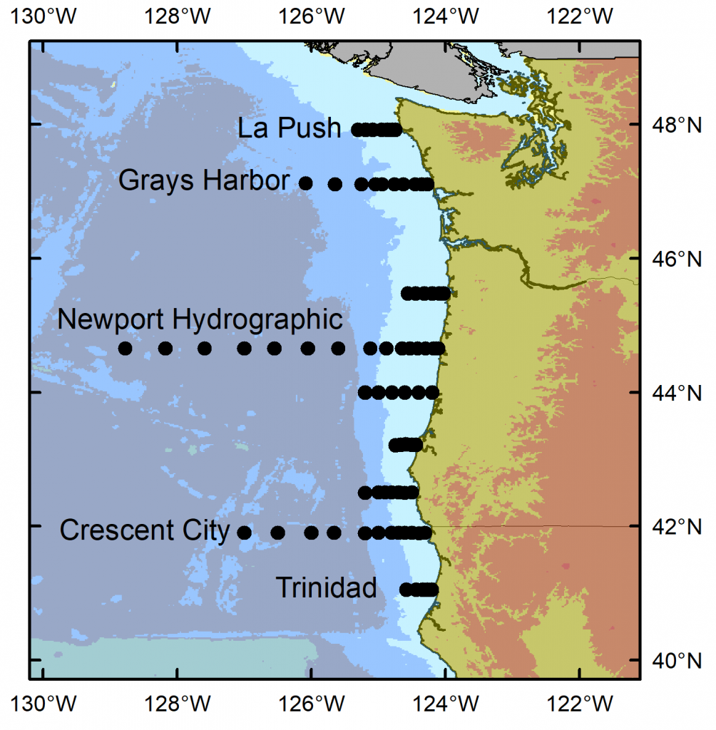
I have just returned from 10 days aboard the NOAA ship Bell M. Shimada, where I was the marine mammal observer on the Northern California Current (NCC) Cruise. These research cruises have sampled the NCC in the winter, spring, and fall for decades. As a result, a wealth of knowledge on the oceanography and plankton community in this dynamic ocean ecosystem has been assimilated by a dedicated team of scientists (find out more via the Newportal Blog). Members of the GEMM Lab have joined this research effort in the past two years, conducting marine mammal surveys during the transits between sampling stations (Fig. 2).
Figure 2. Northern California Current cruise sampling locations, where oceanography and plankton data are collected. Marine mammal surveys were conducted on the transits between stations.
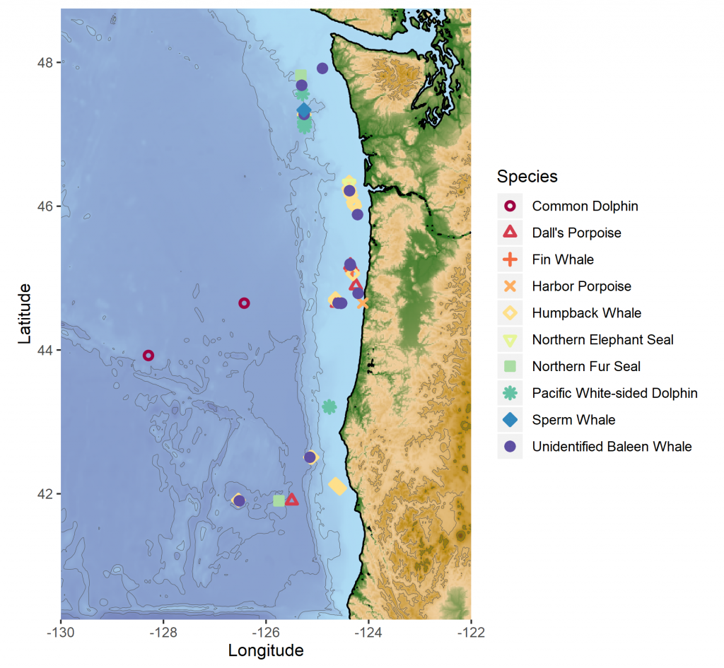
The fall 2019 NCC cruise was a resounding success. We were able to survey a large swath of the ecosystem between Crescent City, CA and La Push, WA, from inshore to 200 miles offshore. During that time, I observed nine different species of marine mammals (Table 1). As often as I use some version of the phrase “the marine environment is patchy and dynamic”, it never fails to sink in a little bit more every time I go to sea. On the map in Fig. 3, note how clustered the marine mammal sightings are. After nearly a full day of observing nothing but blue water, I would find myself scrambling to keep up with recording all the whales and dolphins we were suddenly in the midst of. What drives these clusters of sightings? What is it about the oceanography and prey community that makes any particular area a hotspot for marine mammals? We hope to get at these questions by utilizing the oceanographic data collected throughout the surveys to better understand environmental drivers of these distribution patterns.
Table 1. Summary of marine mammal
sightings from the September 2019 NCC Cruise.
Species
# sightings
Total # individuals
Northern Elephant Seal
1
1
Northern Fur Seal
2
2
Common Dolphin
2
8
Pacific White-sided Dolphin
8
143
Dall’s Porpoise
4
19
Harbor Porpoise
1
3
Sperm Whale
1
1
Fin Whale
1
1
Humpback Whale
22
36
Unidentified Baleen Whale
14
16
Figure 3. Map of marine mammal sighting locations from the September NCC cruise.
It was an auspicious time to survey the Northern California Current. Perhaps you have read recent news reports warning about the formation of another impending marine heatwave, much like the “warm blob” that plagued the North Pacific in 2015. We experienced it first-hand during the NCC cruise, with very warm surface waters off Newport extending out to 200 miles offshore (Fig. 4). A lot of energy input from strong winds would be required to mix that thick, warm layer and allow cool, nutrient-rich water to upwell along the coast. But it is already late September, and as the season shifts from summer to fall we are at the end of our typical upwelling season, and the north winds that would typically drive that mixing are less likely. Time will tell what is in store for the NCC ecosystem as we face the onset of another marine heatwave.
Figure 4. Temperature contours over the upper 150 m from 1-200 miles off Newport, Oregon from Fall 2014-2019. During Fall 2014, the Warm Blob inundated the Oregon shelf. Surface temperatures during that survey were 17°- 18°C along the entire transect. During 2015 and 2016 the warm water (16°C) layer had deepened and occupied the upper 50 m. During 2018, the temperature was 16°C in the upper 20 m and cooler on the shelf, indicative of residual upwelling. During this survey in 2019, we again saw very warm (18°C) temperatures in the upper water column over the entire transect. Image and caption credit: Jennifer Fisher.
It was a joy to spend 10 days at sea with this team of scientists. Insight, collaboration, and innovation are born from interdisciplinary efforts like the NCC cruises. Beyond science, what a privilege it is to be on the ocean with a group of people you can work with and laugh with, from the dock to 200 miles offshore, south to north and back again.
Dawn Barlow on the flying bridge of NOAA Ship Bell M. Shimada, heading out to sea with the Newport bridge in the background. Photo: Anna Bolm.
By: Alexa Kownacki, Ph.D. Student, OSU Department of Fisheries and Wildlife, Geospatial Ecology of Marine Megafauna Lab
Data analysis is often about parsing down data into manageable subsets. My project, which spans 34 years and six study sites along the California coast, requires significant data wrangling before full analysis. As part of a data analysis trial, I first refined my dataset to only the San Diego survey location. I chose this dataset for its standardization and large sample size; the bulk of my sightings, over 4,000 of the 6,136, are from the San Diego survey site where the transect methods were highly standardized. In the next step, I selected explanatory variable datasets that covered the sighting data at similar spatial and temporal resolutions. This small endeavor in analyzing my data was the first big leap into understanding what questions are feasible in terms of variable selection and analysis methods. I developed four major hypotheses for this San Diego site.
The study species: common bottlenose dolphin (Tursiops truncatus) seen along the California coastline in 2015. Image source: Alexa Kownacki.
Hypotheses:
H1: I predict that bottlenose dolphin sightings along the San Diego transect throughout the years 1981-2015 exhibit clustered distribution patterns as a result of the patchy distributions of both the species’ preferred habitats, as well as the social nature of bottlenose dolphins.
H2: I predict there would be higher densities of bottlenose dolphin at higher latitudes spanning 1981-2015 due to prey distributions shifting northward and less human activities in the northerly sections of the transect.
H3: I predict that during warm (positive) El Niño Southern Oscillation (ENSO) months, the dolphin sightings in San Diego would be distributed more northerly, predominantly with prey aggregations historically shifting northward into cooler waters, due to (secondarily) increasing sea surface temperatures.
H4: I predict that along the San Diego coastline, bottlenose dolphin sightings are clustered within two kilometers of the six major lagoons, with no specific preference for any lagoon, because the murky, nutrient-rich waters in the estuarine environments are ideal for prey protection and known for their higher densities of schooling fishes.
Data Description:
The common bottlenose dolphin (Tursiops truncatus) sighting data spans 1981-2015 with a few gap years. Sightings cover all months, but not in all years sampled. The same transect in San Diego was surveyed in a small, rigid-hulled inflatable boat with approximately a two-kilometer observation area (one kilometer surveyed 90 degrees to starboard and port of the bow).
I wanted to see if there were changes in dolphin distribution by latitude and, if so, whether those changes had a relationship to ENSO cycles and/or distances to lagoons. For ENSO data, I used the NOAA database that provides positive, neutral, and negative indices (1, 0, and -1, respectively) by each month of each year. I matched these ENSO data to my month-date information of dolphin sighting data. Distance from each lagoon was calculated for each sighting.
Figure 1. Map representing the San Diego transect, represented with a light blue line inside of a one-kilometer buffered “sighting zone” in pale yellow. The dark pink shapes are dolphin sightings from 1981-2015, although some are stacked on each other and cannot be differentiated. The lagoons, ranging in size, are color-coded. The transect line runs from the breakwaters of Mission Bay, CA to Oceanside Harbor, CA.
Results:
H1:True, dolphins are clustered and do not have a uniform distribution across this area. Spatial analysis indicated a less than a 1% likelihood that this clustered pattern could be the result of random chance (Fig. 1, z-score = -127.16, p-value < 0.0001). It is well-known that schooling fishes have a patchy distribution, which could influence the clustered distribution of their dolphin predators. In addition, bottlenose dolphins are highly social and although pods change in composition of individuals, the dolphins do usually transit, feed, and socialize in small groups.
Figure 2. Summary from the Average Nearest Neighbor calculation in ArcMap 10.6 displaying that bottlenose dolphin sightings in San Diego are highly clustered. When the z-score, which corresponds to different colors on the graphic above, is strongly negative (< -2.58), in this case dark blue, it indicates clustering. Because the p-value is very small, in this case, much less than 0.01, these results of clustering are strongly significant.
H2:False, dolphins do not occur at higher densities in the higher latitudes of the San Diego study site. The sightings are more clumped towards the lower latitudes overall (p < 2e-16), possibly due to habitat preference. The sightings are closer to beaches with higher human densities and human-related activities near Mission Bay, CA. It should be noted, that just north of the San Diego transect is the Camp Pendleton Marine Base, which conducts frequent military exercises and could deter animals.
Figure 3. Histogram comparing the latitudes with the frequency of dolphin sightings in San Diego, CA. The x-axis represents the latitudinal difference from the most northern part of the transect to each dolphin sighting. Therefore, a small difference would translate to a sighting being in the northern transect areas whereas large differences would translate to sightings being more southerly. This could be read from left to right as most northern to most southern. The y-axis represents the frequency of which those differences are seen, that is, the number of sightings with that amount of latitudinal difference, or essentially location on the transect line. Therefore, you can see there is a peak in the number of sightings towards the southern part of the transect line.
H3: False, during warm (positive) El Niño Southern Oscillation (ENSO) months, the dolphin sightings in San Diego were more southerly. In colder (negative) ENSO months, the dolphins were more northerly. The differences between sighting latitude and ENSO index was significant (p<0.005). Post-hoc analysis indicates that the north-south distribution of dolphin sightings was different during each ENSO state.
Figure 4. Boxplot visualizing distributions of dolphin sightings latitudinal differences and ENSO index, with -1,0, and 1 representing cold, neutral, and warm years, respectively.
H4:True, dolphins are clustered around particular lagoons. Figure 5 illustrates how dolphin sightings nearest to Lagoon 6 (the San Dieguito Lagoon) are always within 0.03 decimal degrees. Because of how these data are formatted, decimal degrees is the easiest way to measure change in distance (in this case, the difference in latitude). In comparison, dolphins at Lagoon 5 (Los Penasquitos Lagoon) are distributed across distances, with the most sightings further from the lagoon.
Figure 5. Bar plot displaying the different distances from dolphin sighting location to the nearest lagoon in San Diego in decimal degrees. Note: Lagoon 4 is south of the study site and therefore was never the nearest lagoon.
I found a significant difference between distance to nearest lagoon in different ENSO index categories (p < 2.55e-9): there is a significant difference in distance to nearest lagoon between neutral and negative values and positive and neutral years. Therefore, I hypothesize that in neutral ENSO months compared to positive and negative ENSO months, prey distributions are changing. This is one possible hypothesis for the significant difference in lagoon preference based on the monthly ENSO index. Using a violin plot (Fig. 6), it appears that Lagoon 5, Los Penasquitos Lagoon, has the widest variation of sighting distances in all ENSO index conditions. In neutral years, Lagoon 0, the Buena Vista Lagoon has multiple sightings, when in positive and negative years it had either no sightings or a single sighting. The Buena Vista Lagoon is the most northerly lagoon, which may indicate that in neutral ENSO months, dolphin pods are more northerly in their distribution.
Figure 6. Violin plot illustrating the distance from lagoons of dolphin sightings under different ENSO conditions. There are three major groups based on ENSO index: “-1” representing cold years, “0” representing neutral years, and “1” representing warm years. On the x-axis are lagoon IDs and on the y-axis is the distance to the nearest lagoon in decimal degrees. The wider the shapes, the more sightings, therefore Lagoon 6 has many sightings within a very small distance compared to Lagoon 5 where sightings are widely dispersed at greater distances.
Bottlenose dolphins foraging in a small group along the California coast in 2015. Image source: Alexa Kownacki.
Takeaways to science and management:
Bottlenose dolphins have a clustered distribution which seems to be related to ENSO monthly indices, and likely, their social structures. From these data, neutral ENSO months appear to have something different happening compared to positive and negative months, that is impacting the sighting distributions of bottlenose dolphins off the San Diego coastline. More research needs to be conducted to determine what is different about neutral months and how this may impact this dolphin population. On a finer scale, the six lagoons in San Diego appear to have a spatial relationship with dolphin sightings. These lagoons may provide critical habitat for bottlenose dolphins and/or for their preferred prey either by protecting the animals or by providing nutrients. Different lagoons may have different spans of impact, that is, some lagoons may have wider outflows that create larger nutrient plumes.
Other than the Marine Mammal Protection Act and small protected zones, there are no safeguards in place for these dolphins, whose population hovers around 500 individuals. Therefore, specific coastal areas surrounding lagoons that are more vulnerable to habitat loss, habitat degradation, and/or are more frequented by dolphins, may want greater protection added at a local, state, or federal level. For example, the Batiquitos and San Dieguito Lagoons already contain some Marine Conservation Areas with No-Take Zones within their reach. The city of San Diego and the state of California need better ways to assess the coastlines in their jurisdictions and how protecting the marine, estuarine, and terrestrial environments near and encompassing the coastlines impacts the greater ecosystem.
This dive into my data was an excellent lesson in spatial scaling with regards to parsing down my data to a single study site and in matching my existing data sets to other data that could help answer my hypotheses. Originally, I underestimated the robustness of my data. At first, I hesitated when considering reducing the dolphin sighting data to only include San Diego because I was concerned that I would not be able to do the statistical analyses. However, these concerns were unfounded. My results are strongly significant and provide great insight into my questions about my data. Now, I can further apply these preliminary results and explore both finer and broader scale resolutions, such as using the more precise ENSO index values and finding ways to compare offshore bottlenose dolphin sighting distributions.


You must be logged in to post a comment.