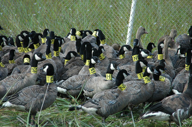
I will (hopefully) be exploring two different data sets in this course. My MS work (described in another post) does not contain any spatially explicit points, so work with programs like Arc becomes more difficult. For several of these analyses I will be using a dataset from the Oregon Department of Fish and Wildlife of cackling goose flock locations.
Cackling geese (Branta hutchinsii minima) are small-bodied geese in the Canada/cackling goose complex (http://www.sibleyguides.com/2007/07/identification-of-cackling-and-canada-goose/). The cackling goose is a is a migratory, Arctic breeding goose with breeding range primarily in the Y-K Delta of Alaska and wintering primarily in Oregon and Washington. Cackling geese are now the most abundant goose species wintering in the Willamette Valley. This follows the general explosion of most Canada goose and cackling goose populations in North America starting around 1966, but the range shift seen in cackling geese is unique coupled with the drastic increase in population size. The cackling goose has increased in number dramatically from an all-time low of less than 20,000 counted in fall surveys during the winter of 1984-85 to over 200,000 birds currently. Along with this population increase has come a change in winter distribution with significantly more use of Oregon and Washington instead of the Central Valley of California, with most birds being found in Oregon’s Willamette Valley and lower Columbia River. To reduce agricultural crop depredation, Oregon refuges have switched to habitat management practices to try and draw cackling geese onto refuge lands. There are also special hunting periods throughout the winter that may influence how flocks use available habitat. Interestingly, cackling geese have consistently been observed increasing their use of urban habitats such as golf courses, parks, sports fields, and residencies.
These birds have been collared on an individual basis since the mid-1990’s. While these data are used largely for mark-recapture analyses to gauge population size, it also produces a large number of flock locations throughout the winter within the Willamette Valley region. Within Oregon, the data spans 1997-2011 and contains 3,141 flock locations with associated latitude/longitude information. These data have been gathered opportunistically by state and federal personnel, and require a bit of data management beforehand.
Using these data, I hope to explore 1) if flock use has changed over the last 20 years, 2) if flock use changes throughout the winter, 3) what habitats feature flocks are most often using (refuge, agricultural, urban), and 4) if flock size changed over time or is influenced by habitat type.
To approach these questions, I would like to conduct several comparable hot spot analyses. I would like to produce a series of maps to provide to ODFW. Understanding flock use is important for resource managers as the population increase pushes birds into private agricultural and urban regions, and if use is changing over time.


It seems like you have a pretty good handle on your data and the direction you’d like to go so I’ll just touch on a few analysis approaches I thought of during your presentation.
First, I thought a could of ways you could address the presence/absence problem. You mention that these data were gathered opportunistically, and in that way they are sort of similar to eBird data. The main difference, as we briefly discussed in class, is that you don’t have observations of other species so you don’t know if someone was looking for other species too and just didn’t find a cackling geese flock. You could assume though, that if two observations were made on the same date and they are near one another, geese were not seen anywhere else in the vicinity. I don’t have any clear idea of the workflow you could use to leverage that idea, but perhaps its worth exploring. If observations were all made along roads and trails, perhaps some kind of network analysis could get at this.
Another way to get around making assumptions about the absence of flocks would be to just count observations per cell. This is what I ended up doing with eBird stuff. You still use the point density tool, but use a square neighborhood shape with a neighborhood size of one cell. This way, you could still do other analyses like comparisons of annual/seasonal distribution changes. It seems this approach works best with a large cell size.
If you set the presence/absence problem aside and use the data as they are I can think of a few ways you might approach the questions you mentioned in your blog post and presentation.
1) To compare any years to one another, perhaps you could calculate density of all points divided by the number of years of observations. This would give you the average density per year. You could then calculate the density for the years of interest and subtract each one from the mean to see where it deviates and how the years differ.
2) Since there seems to be significant differences between months, perhaps whatever comparison you do from year to year should be a comparison of the same month from those two years (e.g. comparing April, 1997 to April 2011.)
3) Cell size is also an important factor for raster analysis. The size of the cell should be determined in part by the maximum radius that an observer could likely see a flock from. You seem well versed with spatial analysis so you probably already know this, but cell alignment is critical for comparing rasters. In Arc you can set a “snap raster” in the environments setting of any tool, and this will ensure that cells are lined up.
4) To analyze differences in land use polygons (urban, refuge, or ag), Zonal Stats seems like a natural choice. It sounds like you were already thinking along these lines though. I don’t know anything about Fragstats but maybe it would be a better approach.