The CGRB will be offering three different workshops this fall. For more information and to register, see the CGRB website.

All workshops are available for credit for students or available to non-students as non-credit workshop(s).

To give perspective students a better insight on each course, we’ve conducted short interviews with the instructors about their course.

See course descriptions and the interviews with the instructors below!


Courses Offered:

Introduction to Unix/Linux and Command-Line Data Analysis (2 modules x 5 weeks @ 2 hrs per week)

Instructor: Matthew Peterson

Course Description:

Introduction to Unix/Linux (5 weeks @ 2 hrs per week)

Logistics:
Date & Time:
Sep 25 – Oct 23, Mon/Wed 2:00pm – 2:50pm
For credit: BDS599 CRN 20579
Workshop Cost: $250


This module introduces the natural environment of bioinformatics: the Linux command line. Material will cover logging into remote machines, filesystem organization and file manipulation, and installing and using software (including examples such as HMMER, BLAST, and MUSCLE). Finally, we introduce the CGRB research infrastructure (including submitting batch jobs) and concepts for data analysis on the command line with tools such as grep and wc.

Command-Line Data Analysis (5 weeks @ 2 hrs per week)

Logistics:
Date & Time: Nov 4  – Dec 4, Mon/Wed, 2:00pm – 2:50pm
For credit: BDS599 CRN 20580
Workshop Cost: $250


The Linux command-line environment has long been used for analyzing text-based and scientific data, and there are a large number of tools pre-installed for data analysis. These can be chained together to form powerful pipelines. Material will cover these and related tools (including grep, sort, awk, sed, etc.) driven by examples of biological data in a problem-solving context that introduces programmatic thinking. This module also covers regular expressions, a useful syntax for matching and substituting string and sequence data.

Matthew Peterson in the CGRB server room

Q1: What do you hope students gain from this workshop?

My hope is that students come to appreciate the power and flexibility of using the text-based command-line interface to interact with (Linux) computational infrastructures. With practice students will become self-sufficient in utilizing the infrastructure to conduct their own research.

Q2: Favorite topic in your course?

Pipelines! The ability to chain the inputs and outputs of multiple commands to filter data is immensely powerful.

Q3: Who should register for this course?

From the first page of the course syllabus: “Linux/Unix Commands, Bioinformatics Utilities, Computational Infrastructure: If you know nothing about the above, then you are exactly in the right course! WELCOME!”

Q4: Advice for users new to bioinformatics and/or programming?

Practice, practice, practice! Learning how to use the command-line effectively is like making a clay pot, you need to get your hands dirty!


RNA-Sequencing (10 weeks @ 2 hrs per week)

Instructor: Dr. Andrew Black

Course Description:

Logistics:
Date & Time: Sept 25 – Dec 5, Tue/Thur 11:00am – 11:50am
For credit: BDS 599, CRN 20581
Workshop Cost: $500

This course provides an introduction to, and practical experience with, the computational component of bulk-RNA-sequencing. After a general overview, participants will obtain a working introduction to command line, R-studio, and accessing and utilizing a computing infrastructure. Students with then work through a series of exercises cleaning raw FASTQ files, aligning reads to a reference genome, quasi-mapping reads to a transcriptome / de novo assembly, followed by data visualization and Differential Gene Expression analysis.

Dr. Andrew Black will teach the RNA-seq workshop this term.

Q1: What do you hope students gain from this workshop?

I hope that students gain an understanding of the computational workflow involved with RNA-seq and an appreciation of the methodology! My overarching goal with this course is that people can use material from this course as scaffolding for analyzing their own data on the CGRB infrastructure.

Q2: Favorite topic in your course?

I added a lord of the rings theme to my course; students are looking for differentially expressed genes between hobbits and golems. I’m a dork, I know, but I had fun spiking different genes into the data and enjoy having students visualize this.

Q3: Who should register for this course?

Graduate students, postdocs, faculty, or anyone outside of OSU that are interested in receiving an introduction to RNA-seq or for those that are needing to learn the workflow for their own project(s).

Q4: Advice for users new to bioinformatics and/or programming?

Take it one step at a time and get comfortable with several commands before expanding your scope. Also, record your commands / code in a text document, because if you aren’t using it on a daily basis, you’ll forget it!


Data Programming in R (6 weeks @ 3 hrs per week)

Instructor: Dr. Shawn O’Neil

Logistics:
Date & Time: Sept. 25 – Nov. 6, Mon/Weds/Fri 9:00am – 9:50am
For credit: ST 599, CRN 17196
Workshop Cost: $500


The R programming language is widely used for the analysis of statistical data sets. This course introduces the language from a computer science perspective, covering topics such as basic data types (e.g. integers, numerics, characters, vectors, lists, matrices, and data frames), importing and manipulating data (in particular, vector and data-frame indexing), control flow (loops, conditionals, and functions), and good practices for producing readable, reusable, and efficient R code. We’ll also explore functional programming concepts and the powerful data manipulation and visualization packages dplyr and tidyr, and ggplot2.

Q1: What do you hope students gain from this workshop?

I really hope that students gain an appreciation for programming as a creative activity. It’s not just a means to an end, even with a statistical language like R; there’s a lot of room for play and exploration. Simulation, for example, is a great way to explore complex systems and ask ‘what if’ questions. Many languages (including R) support programmatic drawing and data visualization which can be quite fun.

Q2: Favorite topic in your course?

I always enjoy the point when we first start scaling analyses to thousands of statistical tests. It’s an eye-opening moment, and doing so in R introduces ‘functional programming,’ a powerful and increasingly important paradigm for software design. 

Q3: Who should register for this course?

Anyone who is interested in doing data analysis, especially of a statistical sort. For those interested in learning programming in a broader sense, our winter Intro to Python series is an excellent overview of fundamental concepts. Although we cover the same topics in the R course, R organizes its features differently than most mainstream programming languages like Python, Java, and C++. Learning both Python and R provides a solid foundation for data science!

Q4: Advice for users new to bioinformatics and/or programming?

I do recommend learning more than one programming language, eventually, as this helps separate deeper concepts from syntax. Find what motivates you and explore it via programming — this could be your primary research project, some field you’ve been wanting to learn more about, or even a hobby. 


This blog post was originally published on September 10, 2018 and written by Christopher M. Sullivan, Assistant Director for Biocomputing. Read the whole article here.

The Oregon State University’s Center for Genome Research and Biocomputing (CGRB) and the Plankton Ecology Lab at OSU Hatfield have been collaborating in implementing an image processing pipeline to automate the classification of in situ images of plankton: microscopic organisms at the base of the food web in the world’s oceans and freshwater ecosystems. The imagery collection from a 10-day cruise typically contains approximately 80 TB worth of video, which, in some cases, may convert into image data yielding several billions of segments representing individual plankton and particles that need to be identified; a near impossible task to carry out manually by human experts. While we have a fully functional Convolutional Neural Net (CNN) algorithm that does an excellent job at predicting the identity of the plankton organisms or particles, we have been limited by GPU computational capabilities. We started working with PCI bus based Tesla K40 and K80 GPUs, which were good enough to manage millions of segments. However, when it came to billions of segments, it became a near insurmountable challenge.

Continue reading

R’s default print function for data frames and matrices is not an effective way to display the contents, especially in a html report. RStudio created a R package, DT, that is an interface to the JavaScript library DataTable. DT allows users to have interactive tables that includes searching, sorting, filtering and exporting! I routinely use these tables in my analysis reports.

Install the DT package from cran

First, one must install and load the DT package. Open up RStudio and run the following commands to install and load the DT package:

# Install the DT package
install.packages("DT")
# Load the DT package
library(DT)

Example Table

The print function is not the most effective was to display a table in an HTML R Markdown report.

print(head(mtcars))
This image has an empty alt attribute; its file name is image-10-1024x252.png

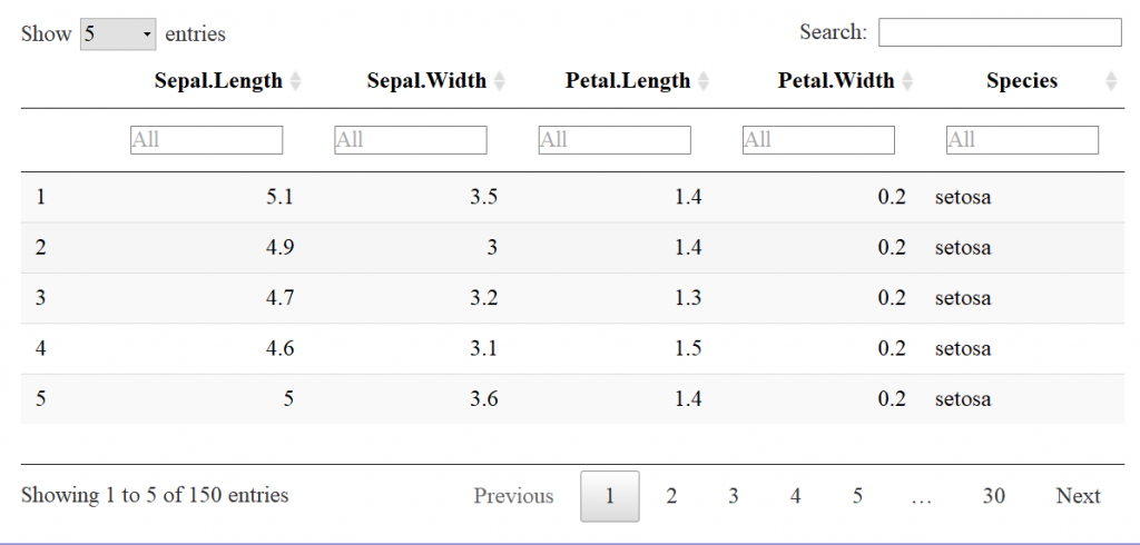
Now let’s look at the datatable function for comparison. The input to the datatable function is a data frame or matrix. Let’s make a table with the preloaded iris data that’s in a data.frame. The basic call is DT::datatable(iris) but in our example I’ve added the filter option to the top of the table, and limited the number of entries to 5 per table. See code and table features below:

datatable(iris, filter = "top", 
          options = list(pageLength = 5))

A screen shot of the output looks like:

This image has an empty alt attribute; its file name is image-1024x490.png

Already, the readability is much better than the base r function print. This is a JavaScript based table, stored in a HTML widget, so a flat image doesn’t convey all of the interactive features.

Features

NUMBER OF ENTRIES TO DISPLAY

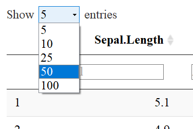
You’ll notice that there is a drop down menu that says: “Show 5 entries”. The default is 10, but I specified 5 as default with the code pageLength=5. One may select the number of entries to show by using the drop down menu like so:

This image has an empty alt attribute; its file name is image-1.png

SEARCH BAR

The widget also includes a search bar on the top right corner which can be very useful when interactively exploring data. Note at the bottom of the table it shows you how many entries (rows) were found and are being displayed.

This image has an empty alt attribute; its file name is image-2.png
This image has an empty alt attribute; its file name is image-3-1024x58.png

SORT COLUMNS

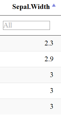
Notice that to the right of each column name are two arrows: One may sort by ascending or descending order and the direction of the blue arrow indicates by which direction you sorted the column.

This image has an empty alt attribute; its file name is image-6.png

FILTER COLUMNS

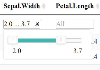
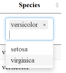
The datatable function also allows users to filter each column depending on the datatype: filter numeric columns with a slider & filter columns of class factor with a drop down menu. One must add the filter = "top" (or bottom, etc.) to the code to enable this feature.

This image has an empty alt attribute; its file name is image-7.png
Numeric columns have sliders
This image has an empty alt attribute; its file name is image-8.png
Columns of class factor have a drop down menu

Export Data

Another useful aspect of the datatable function is the “Buttons” extension. This enables users to copy the table, save as a csv, excel or PDF file, or print the table. The table “remembers” what you’ve changed so far—so if you sort by Sepal Length, filter pedal width to > 1 and select species “versicolor” the copied/saved table will have these same restrictions.

datatable(iris, 
          extensions = 'Buttons',
          options = list(dom = 'Bfrtip', 
                         buttons = c('copy', 'csv', 'excel', 'pdf', 'print'))

The above code adds “buttons” to the top of the table like so:

This image has an empty alt attribute; its file name is image-9.png

If one clicks “copy”, the table will be copied to your clipboard, “CSV” or “PDF” will save the table to the give file type, and “print” will bring put the table into a print friendly format and will bring up the print dialog box.

Links and Color

One may also have links in their table. Say you made a data frame with links you want to work in your html report. For example: a data frame of variants w/ links to their position in a genome browser. This is done through not escaping content in the table, specifically the column with the links. The links are made with html and must not be escaped to show up. This applies to other html as well; including color. For me, it was confusing that I had to not escape the html columns. Got it completely backwards the first time I tried it. NOTE: > got replaced with “& gt;” (with no spaces) when it is rendered on the blog… Need to find a fix!

# Make dataframe
df.link <- data.frame(school=c("OSU", "UO", "Linfield", "Willamette"), 
                      mascot=c("beavers", "ducks", "wildcats", "bearcats"),
                      website=c('<a href="http://oregonstate.edu/">oregonstate.edu</a>',
                                '<a href="https://www.uoregon.edu/">uoregon.edu</a>',
                                '<a href="https://www.linfield.edu/">linfield.edu</a>',
                                '<a href="https://www.willamette.edu/">willamette.edu</a>'),
                      School_colors=c('<span style="color:orange">orange & black</span>', 
                                        '<span style="color:green">green & yellow</span>', 
                                        '<span style="color:purple">purple and red</span>', 
                                        '<span style="color:red">red and yellow</span>'))

# When the html columns, 3 & 4, are not escaped, it works!
datatable(df.link, escape = c(1,2,3))
This image has an empty alt attribute; its file name is image-11-1024x333.png

Column Visibility

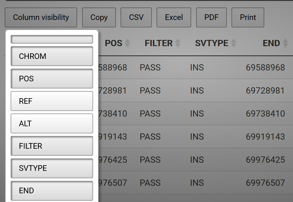
One may also hide columns from visibility and add a button to add the column back interactively. For example, say we have a data frame called sv.all.i.in. We can hide columns 3 and 4, which are long sequences and disrupt the readability of the table, with the following code:

datatable(sv.all.i.in, extensions = 'Buttons',
          options = list(dom = 'Bfrtip', columnDefs = list(list(visible=FALSE, targets=c(3,4))), 
                         buttons = list(I('colvis'),c('copy', 'csv', 'excel', 'pdf', 'print'))))
This image has an empty alt attribute; its file name is image-12.png

Learn More

There are many more useful features that you can add to your datatable! Learn more here: https://rstudio.github.io/DT/